Cell Search

Introduction

When a User Equipment(UE) is powered on or when it enters a new cell, it must be able to find the cell and synchronize to it in frequency and time. It must also be able to read some system information describing the cell in order to see if it can be used by the UE.

5G NR uses below synchronization signals:

  • Primary Synchronization Signal, PSS, with 3 different code sequences
  • Secondary Synchronization Signal, SSS, with 336 different code sequences

These signals enable the UE to find a cell along with helping it in synchronizing to the cell’s timing. There can be 1008 (3 X 336) possible code sequences and the value in the PSS/SSS determines cell’s Physical Cell Identity (PCI). When the UE finds these synchronization signals, it can also read the Physical Broadcast Channel (PBCH), whose location can be found around these synchronization signals.

Cell search also covers the functions and procedures by which a device finds new cells. The procedure is carried out when a device is initially entering the coverage area of a system. To enable mobility, cell search procedure is also continuously carried out by devices moving within the system, both when the device is connected to the network and when in idle/inactive state.

Cell Search in Standalone Mode

In order to perform the initial cell access in the Standalone (SA) mode, a UE need to perform Contention Based Random Access procedure (CBRA) and therefore it needs to acquire the relevant system information, which is System Information Block1 (SIB1). Accessing this information requires acquisition of Master Information Block (MIB) and it’s decoding. This is only possible while detecting and identifying the synchronization signal block. However, no information is provided in the SA mode to find the frequencies where the SSBs are transmitted, unlike Non-Standalone (NSA) mode where the UE receives the exact frequency location of the SSB via dedicated RRC signaling over the established LTE connection.

Synchronization Signal Block

A synchronization signal block (SSB) consists of one OFDM symbol for the PSS and one OFDM symbol for the SSS. Furthermore, the SS block may contain two OFDM symbols for the PBCH which are identical. So, the SS block spans four OFDM symbols in the time domain and 240 subcarriers in the frequency domain. PSS is transmitted in the first OFDM symbol of the SS block and occupies 127 subcarriers in the frequency domain. The remaining subcarriers are empty. SSS is transmitted in the third OFDM symbol of the SS block and occupies the same set of subcarriers as the PSS. There are eight and nine empty subcarriers on each side of the SSS. PBCH is transmitted within the second and fourth OFDM symbols of the SS block. In addition, PBCH transmission also uses 48 subcarriers on each side of the SSS. The total number of resource elements used for PBCH transmission per SS block thus equals 576, which includes resource elements for the PBCH along with resource elements for the demodulation reference signals (DMRS) needed for coherent demodulation of the PBCH.

Structure of SS Block

The synchronization signals and the physical broadcast channel within a synchronization signal block are time multiplexed. Below fig. shows another way of representing structure of SSB.

Synchronization signal block

One important difference between the SS block and the corresponding signals for LTE is the possibility to apply beam-sweeping for SS-block transmission i.e. the possibility to transmit SS blocks in different beams in a time-multiplexed fashion.

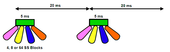
The timing of the SS Block can be set by the network operator. Default value of SSB transmission is 20ms but can be set between 5 and 160ms (5, 10, 20, 40, 80 and 160). During this time set by the operator, a number of SS Blocks will be transmitted in different directions (called Beams) during a 5ms Period. Each block of transmitted SS Blocks is referred to as an SS Burst Set. Although the periodicity of the SS burst set is flexible with a minimum period of 5ms and a maximum period of 160ms, each SS burst set is always confined to a 5ms time interval, either in the first or second half of a 10ms frame. Below example shows the default setting of 20ms.

Example of SS Block Timing with default setting

By applying beamforming for the SS block, the coverage of a single SS block transmission gets increased. Beam-sweeping for SS-block transmission also enables receiver-side beam-sweeping for the reception of uplink random-access transmissions as well as downlink beamforming for the random-access response

Now, the 20ms SS-block periodicity is four times longer than the corresponding 5ms periodicity of LTE PSS/SSS transmission. The longer SS-block period was selected to allow for enhanced NR network energy performance and in general to follow the ultra-lean design paradigm. The drawback with a longer SS-block period is that a device must stay on each frequency for a longer time in order to conclude that there is no PSS/SSS on the frequency. However, this is compensated for by the sparse synchronization raster which reduces the number of frequency-domain locations on which a device must search for an SS block.

SS Blocks can be sent over 4, 8 or 64 beams in a cell. The lower numbers will be used for lower frequencies as there will be a smaller number of antennas for such configuration. The SS Blocks will be used as follows:

  • 4 SS Blocks: used for frequency range 1 below 3 GHz
  • 8 SS Blocks: used for frequency range 1 between 3 and 6 GHz
  • 64 SS Blocks: used for frequency range 2

As per specifications, there can be different cases for the SS Block transmission. These cases cover different sub carrier spacings along with normal or extended cyclic prefix if the subcarrier spacing used is 30KHz. These cases are depicted below in the fig:

Different cases of SS Block Transmission

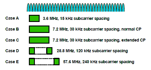
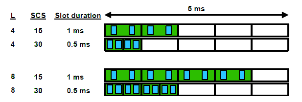
As you would have noticed, 60KHz subcarrier spacing is not included in above cases since it can’t carry any SS Blocks. Also, note that an SS Block is always distributed over 20 resource blocks in frequency domain. The size of the SS Block in the frequency domain will scale as per the subcarrier spacing used. Not all slots can be used for transmission of the block during the 5ms period when SS block can be transmitted. The number of slots used will also depend on the number of transmissions (4, 8 or 64) during the 5ms period. Below fig shows the possible transmission of SS Blocks for the case of 4 and 8 transmission times per 5ms period (depicted by the ‘L’ parameter in below fig)

Different options of SS Block Configuration

Difference between LTE and NR Cell Search Approach

In LTE, synchronization signals were located in the center of transmission BW so once an LTE device has found a PSS/SSS i.e. found a carrier, it inherently knows the center frequency of the found carrier. The drawback was that a device with no prior knowledge of the frequency-domain carrier position must search for PSS/SSS at all possible carrier positions (the “carrier raster”). So, a different approach has been adopted in 5G, to allow for faster cell search. In 5G, the signals are not fixed, rather located in a synchronization raster (a more limited set of possible locations of SS block within each frequency band). Instead of searching for an SS block at each position of the carrier raster, a device only needs to search for an SS block on the sparse synchronization raster. When found, the UE gets informed on where in frequency domain it is located.

Also, LTE used a concept of 2 synchronization signals with a fixed format which enabled UEs to find a cell. 5G NR also uses 2 synchronization signals but the difference is the support of beamforming and reduction in the number of “Always on” signals.

PSS and SSS

PSS is the first signal that a device entering the system will search for. At that stage, the device has no knowledge of the system timing. Once the device has found the PSS, it has found synchronization up to the periodicity of the PSS. PSS extends over 127 resource elements and has 3 different PSS Sequences. Physical cell identity (PCI) of the cell determines which of the three PSS sequences to use in a certain cell. When searching for new cells, a device must search for all three PSSs.

Once a device detects a PSS it knows the transmission timing of the SSS. By detecting the SSS, the device can determine the PCI of the detected cell. There are 1008 (3 X 336) different PCIs. However, already from the PSS detection the device has reduced the set of candidate PCIs by a factor 3. There are thus 336 different SSSs, that together with the already-detected PSS provides the full PCI. The basic structure of the SSS is same as that of the PSS i.e. the SSS consists of 127 subcarriers to which an SSS sequence is applied.

PBCH

While the PSS and SSS are physical signals with specific structures, PBCH is a more conventional physical channel on which explicit channel-coded information is transmitted. PBCH carries the MIB, which contains information that the device needs in order to be able to acquire the remaining SI broadcast by the network.

Below table shows the information carried by the PBCH:

Different options of SS Block Configuration
PBCH Contents
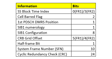
  • SS-block time index identifies the SS-block location within an SS burst set. Each SS block has a well-defined position within an SS burst set which is contained within the first or second half of a 5ms frame. From the SS-block time index, in combination with the half-frame bit, the device can determine the frame boundary. The SS-block time index is provided to the device as two parts:
    • 1st part encoded in the scrambling applied to the PBCH
    • 2nd part included in the PBCH payload.

For operation in higher NR frequency range (FR2), there can be up to 64 SS blocks within an SS burst set, implying the need for 3 additional bits to indicate the SS-block time index. These 3 bits are only needed for operation above 10 GHz and are included as explicit information within the PBCH payload.

  • CellBarred flag consist of two bits where 1st bit is the actual CellBarred flag that indicates whether devices can access the cell or not. Assuming devices are not allowed to access the cell, the 2nd bit, also referred to as the Intra-frequency-reselection flag, indicates whether access is permitted to other cells on the same frequency or not.
  • 1st PDSCH DMRS position indicates the time-domain position of the first DMRS symbol assuming DMRS Mapping Type A
  • SIB1 numerology provides info about the subcarrier spacing used for the transmission of the SIB1. The same numerology is also used for the downlink Message 2 and Message 4 that are part of the random-access procedure.
  • SIB1 configuration provides info about the search space, corresponding CORESET, and other PDCCH-related parameters that a device needs in order to monitor for the scheduling of SIB1.
  • CRB grid offset provides info about the frequency offset between the SS block and the common resource block grid. Information about the absolute position of the SS block within the overall carrier is provided within SIB1.
  • Half-frame bit indicates if the SS block is located in the 1st or 2nd 5ms part of a 10ms frame.

Acquiring System Information

When the UE has found the SS Block, it can read the PBCH which contains MIB. When the MIB has been decoded by the UE, it can start to search for SIB1. When SIB1 has been found and read, all remaining SIBs are decoded or requested.

In LTE, all system information was periodically broadcast over the entire cell area making it always available but also implying that it is transmitted even if there is no device within the cell. 5G NR, on the other hand, adopted a different approach where the system information, beyond the very limited information carried within the MIB, has been divided into two parts: SIB1 and the remaining SIBs.

SIB1 which is sometimes also referred to as the remaining minimum system information (RMSI) consists of the system information that a device needs to know before it can access the system. SIB1 is always periodically broadcast over the entire cell area. One important task of SIB1 is to provide the information the device needs in order to carry out an initial random access. SIB1 is provided by means of ordinary scheduled PDSCH transmissions with a periodicity of 160ms. The PBCH/MIB provides information about the numerology used for SIB1 transmission as well as the search space and corresponding CORESET used for scheduling of SIB1. Within that CORESET, the device then monitors for scheduling of SIB1 indicated by a special System Information RNTI (SI-RNTI).

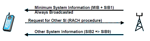
In 5G a UE can request for other system information with a RACH procedure, as compared to the traditional mobile networks, where all other system information (SIB =>) is broadcasted. Below is the terminology that is used in 5G for the system information:

  • Minimum System Information
    • Master Information Block (MIB)
    • System Information Block1 (SIB1)
  • Other System Information
    • System Information Block 2 to 9 (SIB2 to SIB9)
Transmission of System Information

Minimum SI is always broadcasted in the whole cell. When Beamforming is used, the information is transmitted in all the beams. If a UE can’t decode the minimum SI, it should regard the cell as barred for access or camping.

Note: Small micro or Pico cells may not be used for initial access so the UEs must use a large macro cell for access and camping. The smaller cells may only be activated on demand when the traffic is high.

Other SI can be broadcasted but not always. This can be used in larger cells with high traffic.

As mentioned earlier, it is possible to request the other SI on-demand, which can be used in cells with low traffic. To request for the SI, the UE need to perform random access procedure. The network can either reserve dedicated resources for this request, or the UE will indicate the request for other system information in the message sent to the network. This way the network can avoid periodic broadcast of these SIBs in cells where no device is currently camping, thereby allowing for enhanced network energy performance.

Below is the short summary of the information carried by different SIBs:

  • SIB1: PLMN identity list, Tracking Area Code, Cell Identity, Barred/not Barred Indication, Cell Selection Information, SI scheduling information, support for emergency call indication, support for IMS voice call indication, timers, constants, barring information
  • SIB2: Cell reselection information
  • SIB3: Neighboring cells on same frequency (5G)
  • SIB4: Neighboring cells on different frequency (5G)
  • SIB5: Neighboring LTE cells
  • SIB6/7: ETWS information (Earthquake and Tsunami warning system)
  • SIB8: CMAS (Commercial Mobile Alert System)
  • SIB9: GPS and UTC Time

References:

  1. “5G NR – The next generation wireless access technology” – By Erik Dahlman, Stefan Parkvall, Johan Sköld
  2. http://www.techplayon.com/5g-nr-cell-search-and-synchronization-acquiring-system-information/
  3. http://howltestuffworks.blogspot.com/2019/10/5g-nr-synchronization-signalpbch-block.html

Carrier Aggregation

Introduction

Carrier Aggregation is a technology that aggregates multiple component carriers (CC), which can be jointly used for transmission to/from a single device. It combines two or more carriers into one data channel to enhance the data capacity of a network. Using existing spectrum, Carrier Aggregation helps mobile network operators (MNOs) in providing increased UL and DL data rates. When Carrier Aggregation is deployed, frame timing and SFN are aligned across cells that can be aggregated. 5G NR utilizes CA in both FR1 and FR2, supporting up to 16 component carriers. For Release 15, the maximum number of configured Component Carriers for a UE is 16 for DL and 16 for UL.

Important characteristics:

  • Up to 16 carriers (contiguous and non-contiguous) can be aggregated
  • Carriers can use different numerologies
  • Transport block mapping is per carrier
  • Cross carrier scheduling and joint feedback are also supported
  • Flexibility for network operators to deploy their licensed spectrum by using any of the CA types (such as intra-band contiguous, intra-band noncontiguous or inter-band noncontiguous)

History

LTE release 10 introduced enhanced LTE spectrum flexibility through carrier aggregation which was required to support higher bandwidths and fragmented spectra. Up to 5 component carriers, possibly each of different bandwidth, can be aggregated in this release, allowing for transmission bandwidths of up to 100MHz.  All component carriers need to have the same duplex scheme and in the case of TDD, same uplink downlink configuration.

In LTE release 10, Backwards compatibility was ensured as each component carrier uses the release-8 structure. Hence, to a release-8/9 device each component carrier will appear as an LTE release-8 carrier, while a carrier-aggregation capable device can exploit the total aggregated bandwidth, enabling higher data rates. In the general case, a different number of component carriers can be aggregated for the downlink and uplink. This was an important property from a device complexity point of view where aggregation can be supported in the downlink where very high data rates are needed without increasing the uplink complexity.

Release 13 marked the start of LTE Advanced Pro, included various enhancements in Carrier Aggregation. The number of component carriers possible to aggregate was increased to 32, resulting in a total bandwidth of 640MHz and a theoretical peak data rate around 25 Gbit/s in the DL considering 8 layers spatial multiplexing and 256 QAM. The main motivation for increasing the number of subcarriers was to allow for very large bandwidths in unlicensed spectra.

LTE release 13 also introduced license-assisted access, where the carrier aggregation framework is used to aggregate downlink carriers in unlicensed frequency bands, primarily in the 5 GHz range, with carriers in licensed frequency bands. Mobility, critical control signaling and services demanding high quality-of-service rely on carriers in the licensed spectra while (parts of) less demanding traffic can be handled by the carriers using unlicensed spectra.

In LTE release 14, license-assisted access was enhanced to address uplink transmissions also.

Carrier aggregation was one of the most successful enhancements of LTE till now with new combinations of frequency band added in every release.

Carrier Aggregation in NR

Like LTE, multiple NR carriers can be aggregated and transmitted in parallel to/from the same device, thereby allowing for an overall wider bandwidth and correspondingly higher per-link data rates. The carriers do not have to be contiguous in the frequency domain but can be dispersed, both in the same frequency band as well as in different frequency bands, resulting in three difference scenarios:

Intraband aggregation with frequency-contiguous component carriers;

Intraband aggregation with non-contiguous component carriers;

Interband aggregation with non-contiguous component carriers.

Below figure depicts these 3 scenarios:

Carrier Aggregation Types

Although the overall structure is the same for all three cases, the RF complexity can be vastly different.

Up to 16 carriers, having different bandwidths and different duplex schemes, can be aggregated allowing for overall transmission bandwidths of up to 6,400 MHz (16 x 400 MHz) = 6.4 GHz, which is more than typical spectrum allocations.

A device capable of CA may receive or transmit simultaneously on multiple component carriers while a device not capable of CA can access one of the component carriers. It is worth noting that in the case of Inter-band carrier aggregation of multiple half-duplex (TDD) carriers, the transmission direction on different carriers does not necessarily have to be the same. This implies that a carrier-aggregation-capable TDD device may need a duplex filter, unlike the typical scenario for a noncarrier-aggregation-capable device.

In the specifications, carrier aggregation is described using the term cell, that is, a carrier-aggregation-capable device can receive and transmit from/to multiple cells. One of these cells is referred to as the primary cell (PCell). This is the cell which the device initially finds and connects to, after which one or more secondary cells (SCells) can be configured, once the device is in connected mode. The secondary cells can be rapidly activated or deceived to meet the variations in the traffic pattern. Different devices may have different cells as their primary cell—that is, the configuration of the primary cell is device-specific. Furthermore, the number of carriers (or cells) does not have to be the same in UL and DL. In fact, a typical case is to have more carriers aggregated in the DL than in the UL. Reasons being:

  • There is typically more traffic in the DL that in the UL.
  • The RF complexity from multiple simultaneously active uplink carriers is typically larger than the corresponding complexity in the downlink.

Carrier aggregation uses L1/L2 control signaling for the same reason as when operating with a single carrier. As baseline, all the feedback is transmitted on the primary cell, motivated by the need to support asymmetric carrier aggregation with the number of downlink carriers supported by a device different than the number of uplink carriers. For many downlink component carriers, a single uplink carrier may carry a large number of acknowledgments. To avoid overloading a single carrier, it is possible to configure two PUCCH groups where feedback relating to the first group is transmitted in the uplink of the PCell and feedback relating to the other group of carriers is transmitted on the primary second cell (PSCell).

Multiple PUCCH Groups

If carrier aggregation is used, the device may receive and transmit on multiple carriers, but reception on multiple carriers is typically only needed for the highest data rates. It is therefore beneficial to inactivate reception of carriers not used while keeping the configuration intact. Activation and inactivation of component carriers can be done through MAC signaling containing a bitmap where each bit indicates whether a configured SCell should be activated or deactivated.

Difference between self-scheduling and cross-carrier scheduling

Scheduling grants and scheduling assignments can be transmitted on either the same cell as the corresponding data, known as self-scheduling, or on a different cell than the corresponding data, known as cross-carrier scheduling.

Self-scheduling vs Cross-scheduling

Let’s discuss in detail – the scheduling decisions are taken per carrier and the scheduling assignments are transmitted separately for each carrier, that is, a device scheduled to receive data from multiple carriers simultaneously receives multiple PDCCHs. A PDCCH received can either point to the same carrier, known as self-scheduling, or to another carrier, commonly referred to as cross-carrier scheduling or cross-scheduling. In case of cross-carrier scheduling of a carrier with a different numerology than the one upon which the PDCCH was transmitted, timing offsets in the scheduling assignment, for example, which slot the assignment relates to, are interpreted in the PDSCH numerology (and not the PDCCH numerology).

Carrier Aggregation support in MAC Layer

MAC Layer is responsible for multiplexing/demultiplexing data across multiple component carriers when carrier aggregation is used. In case of CA, it is responsible for distributing data from each flow across the different component carriers, or cells.

The basic principle for carrier aggregation is independent processing of the component carriers in the physical layer, including control signaling, scheduling and HARQ retransmissions, while carrier aggregation is invisible above the MAC layer. Carrier aggregation is therefore mainly seen in the MAC layer, where logical channels, including any MAC control elements, are multiplexed to form transport blocks per component carrier with each component carrier having its own HARQ entity.

Carrier Aggregation in MAC

Note: In the case of carrier aggregation, there is one DL-SCH (or UL-SCH) per component carrier seen by the device

Relation with Dual Connectivity

Dual connectivity implies that a device is simultaneously connected to two cells. User-plane aggregation, where the device is receiving data transmission from multiple sites, separation of control and user planes, and uplink-downlink separation where downlink transmissions originate from a different node than the uplink reception node are some examples of the benefits with dual connectivity. To some extent it can be seen as carrier aggregation extended to the case of non-ideal backhaul. It is also essential for NR when operating in non-standalone mode with LTE providing mobility and initial access.

Example of Dual Connectivity

In dual connectivity, a device is connected to two cells, or in general, two cell groups, the Master Cell Group (MCG) and the Secondary Cell Group (SCG). The reason for the term cell group is to cover also the case of carrier aggregation where there are multiple cells, one per aggregated carriers, in each cell group. The two cell groups can be handled by different gNBs.

Dual Connectivity Details

A radio bearer is typically handled by one of the cell groups, but there is also the possibility for split bearers, in which case one radio bearer is handled by both cell groups. In this case, PDCP is in charge of distributing the data between the MCG and the SCG and thus PDCP plays an important role for Dual connectivity support.

Differences between Dual Connectivity and Carrier Aggregation

Both carrier aggregation and dual connectivity result in the device being connected to more than one cell. Despite this similarity, there are fundamental differences, primarily related to how tightly the different cells are coordinated and whether they reside in the same or in different gNBs.

Carrier aggregation implies very tight coordination, with all the cells belonging to the same gNB. Scheduling decisions are taken jointly for all the cells the device is connected to by one joint scheduler. Dual connectivity, on the other hand, allows for a much looser coordination between the cells. The cells can belong to different gNBs, and they may even belong to different radio-access technologies as is the case for NR-LTE dual connectivity in case of non-standalone operation.

Carrier aggregation and dual connectivity can also be combined. This is the reason for the terms master cell group and secondary cell group. Within each of the cell groups, carrier aggregation can be used.

Multi Connectivity includes Dual Connectivity (PDCP UP Split) and Carrier Aggregation (MAC UP Split) as shown in the figure below:

Carrier Aggregation with Dual Connectivity

Dual Connectivity should be preferred when latency is not neglectable between paths i.e. > 5-10ms or when there is a different RAT to be connected and TN of the master side is congested, whereas Carrier Aggregation has better and faster utilization of radio resources than Dual Connectivity but is used to connect same RATs. It requires low inter site latency (<5ms).

Note:

  • In the case of carrier aggregation or dual connectivity, multiple power headroom reports can be contained in a single message (MAC control element).
  • NR does not support carrier aggregation with LTE and thus dual connectivity is needed to support aggregation of the LTE and NR throughput.
  • NR specifications supports carrier aggregation, where multiple carriers are present within a band, or in multiple bands, can be combined to create larger transmission bandwidths.

Relation with Supplementary Uplink

Both these techniques allow the uplink transmission to be switched between the FDD-band and the 3.5 GHz band. The use of these mechanisms effectively utilizes idle sub-3 GHz band resources, improve the uplink coverage of C-band, and enable the provisioning of 5G services in a wider area. Both solutions, NR Carrier Aggregation and Supplementary Uplink, offer transport of UL user data using sub-3GHz band NR radio resources. NR CA provides the added benefit of also providing sub-3GHz DL user data support on the FDD-band downlink, using 3GPP specified LTE-NR spectrum sharing, if needed. This provides opportunity to aggregate NR bandwidth as well as better operation of the NR uplink.

Difference between Carrier Aggregation (CA) and supplementary uplink (SUL)

Supplementary uplink differs from the aggregated uplink in that the UE may be scheduled to transmit either on the supplementary uplink or on the uplink of the carrier being supplemented, but not on both at the same time.

In a typical carrier aggregation scenario:

  • Main aim of carrier aggregation is to enable higher peak data rates by increasing the bandwidth available for transmission to/from a device.
  • The two (or more) carriers are often of similar bandwidth and operating at similar carrier frequencies, making aggregation of the throughput of the two carriers more beneficial. Each uplink carrier is operating with its own associated downlink carrier, simplifying the support for simultaneous scheduling of multiple uplink transmissions in parallel. Formally, each such downlink carrier corresponds to a cell of its own and thus different uplink carriers in a carrier-aggregation scenario correspond to different cells.

While in case of SUL scenario:

  • Main aim of SUL is to extend uplink coverage, that is, to provide higher uplink data rates in power-limited situations, by utilizing the lower path loss at lower frequencies
  • The supplementary uplink carrier does not have an associated downlink carrier of its own. Rather, the supplementary carrier and the conventional uplink carrier share the same downlink carrier.  Consequently, the supplementary uplink carrier does not correspond to a cell of its own. Instead, in the SUL scenario there is a single cell with one downlink carrier and two uplink carriers.
Carrier Aggregation vs Supplementary Uplink

Benefits of Carrier Aggregation

  • Better Network Performance: Carriers provide a more reliable and stronger service with less strain on individual networks.
  • Leveraging of underutilized spectrum: CA enables carriers to take advantage of underutilized and unlicensed spectrum, thereby extending the benefits of 5G NR to these bands.
  • Increased uplink and downlink data rates: Wider bandwidth mean higher data rates.
  • More efficient use of spectrum: Operators can combine fragmented smaller spectrum holdings into larger and more useful blocks and can create aggregated bandwidths greater than those that would be possible from a single component carrier.
  • Network carrier load balancing: Enables intelligent and dynamic load balancing with real‐time network load data.
  • Higher capacity: CA doubles the data rate for users while reducing latency with a good amount.
  • Scalability: Expanded coverage allows carriers to scale their networks rapidly.
  • Dynamic switching: CA enables dynamic flow switching across component carriers (CCs).
  • Better user experience: CA delivers a better user experience with higher peak data rates (particularly at cell edges), higher user data rates, and lower latency, as well as more capacity for “bursty” usage such as web browsing and streaming video.
  • Enabling of new mobile services: Delivering a better user experience opens opportunities for carriers to innovate and offer new high bandwidth/high data rate mobile services.
  • Can be combined with Dual Connectivity

Disadvantages/Challenges with Carrier Aggregation:

  • Intra‐band uplink CA signals use more bandwidth and have higher peak‐to‐average power ratios (PAPRs)
  • Many possible configurations of resource blocks (RBs) exist in multiple component carriers (CCs) where signals could mix and create spurious out‐of‐band problems.
  • Intra‐band CA signals present mobile device designers with many challenges because they can have higher peaks, more signal bandwidth, and new RB configurations. A Power Amplifier design must be tuned for very high linearity even though the signal power may be backed off. Adjacent channel leakage, intermodulation products of non‐contiguous RBs, spurious emissions, noise, and sensitivity must be considered. The tradeoff of linearity comes at the expense of efficiency and thermal effects.
  • Inter‐band CA combines transmit signals from different bands. The maximum total power transmitted from a mobile device is not increased in these cases, so for two transmit bands, each band carries half the power of a normal transmission, or 3 dB less than a non‐CA signal. Because different PAs are used to amplify the signals in different bands, and the transmit power is reduced for each, the PA linearity isn’t an issue. Other front‐end components, like switches, have to deal with high‐level signals from different bands that can mix and create intermodulation products. These new signals can interfere with one of the active cellular receivers or even another receiver on the phone, like the GPS receiver. To manage these signals, switches must have very high linearity.

References:

  1. https://www.gsma.com/futurenetworks/wp-content/uploads/2019/03/5G-Implementation-Guideline-v2.0-July-2019.pdf
  2. “5G NR – The next generation wireless access technology” – By Erik Dahlman, Stefan Parkvall, Johan Sköld
  3. https://www.3gpp.org/technologies/keywords-acronyms/101-carrier-aggregation-explained
  4. https://www.qorvo.com/design-hub/ebooks/5g-rf-for-dummies

HARQ

Introduction

5G NR (New radio) has several retransmission systems using three different layers in the protocol stack:

  • MAC protocol: It implements a fast retransmission system with delay less than 1ms in new radio, called HARQ (Hybrid Automatic Repeat reQuest).
  • RLC protocol: Even though HARQ is present at MAC but there might still be some possibility of errors in the feedback system. So, for dealing with those errors, RLC has a slow retransmission system but with a feedback protected by CRC. Compared to the HARQ acknowledgments, the RLC status reports are transmitted relatively infrequently.
  • PDCP protocol: This will guarantee in-sequence delivery of user data and it is mainly used during handover as RLC and MAC buffers are flushed when a handover is executed.

NR uses an asynchronous hybrid-ARQ protocol in both downlink and uplink, that is, the hybrid-ARQ process which the downlink or uplink transmission relates to is explicitly signaled as part of the downlink control information (DCI). The hybrid-ARQ mechanism in the MAC layer targets very fast retransmissions and, consequently, feedback on success or failure of the downlink transmission is provided to the gNB after each received transport block (for uplink transmission no explicit feedback needs to be transmitted as the receiver and scheduler are in the same node).

HARQ is implemented to correct the erroneous packets coming from PHY layer. If the received data is erroneous then the receiver buffers the data and requests for a re-transmission from the sender. When the receiver receives the re-transmitted data, it then combines it with buffered data prior to channel decoding and error detection. This helps in the performance of re-transmissions. For this to work, the sending entity need to buffer the transmitted data until the ACK is received since the data needs to be retransmitted in case a NACK is received.

HARQ is a stop and wait (SAW) protocol with multiple processes. The protocol will continue to repair one transmission without hindering other ongoing transmissions which can continue in parallel.

HARQ principle with multiple processes

Why multiple SAW processes are required?

Once a packet is sent from a process, it waits for an ACK/NACK. While it is waiting for an ACK/NACK in the active state, no other work can be done by the same process leading to reduced performance. So, if we have multiple such processes working in parallel, throughput can be increased by making other processes work at the same time on other packets, while a process is in waiting state for ACK/NACK.

Differences with LTE HARQ

  • New radio is using an asynchronous protocol in both UL and DL, which is different from LTE, where the protocol was synchronous in UL; UE should reply with an ACK/NACK after 3ms of receiving the DL data. The gNB knows that when the ACK/NACK is expected. In NR, the report timing is not fixed to increase the flexibility which is important for URLLC services.
  • PHICH (Physical HARQ Indicator channel) was used in LTE to handle uplink retransmissions and was tightly coupled to the use of a synchronous HARQ protocol, but since the NR HARQ protocol is asynchronous in both uplink and downlink the PHICH is not needed in NR.
  • In LTE, Non-adaptive retransmissions were triggered by a negative acknowledgement on the PHICH, which used the same set of resources as the previous transmission i.e. the modulation scheme and the set of allocated resource blocks remains unchanged. Only Redundancy version used to change between transmissions. But in NR, PHICH is not there and retransmissions are adaptive that can be triggered by DCI. NDI flag retriggers a transmission if its value is toggled relative to previous transmission.
  • Maximum number of HARQ processes was set to 8 in LTE but is increased to 16 in NR. This was motivated by shorter time slot and increased use of remote radio heads that will increase the round-trip time slightly.

Reasons why NR HARQ is asynchronous in both UL and DL:

  • Synchronous HARQ operation does not allow dynamic TDD.
  • Operation in unlicensed spectra (part of later NR releases) is more efficient with asynchronous operation as it is not guaranteed that the radio resources are available at the time for a synchronous transmission.

Hybrid ARQ with Soft combining

The hybrid-ARQ protocol is the primary way of handling retransmissions in NR. In case of an erroneously received packet, a retransmission is requested. However, despite it not being possible to decode the packet, the received signal still contains information, which is lost by discarding erroneously received packets. This shortcoming is addressed by hybrid-ARQ with soft combining. In hybrid- ARQ with soft combining, the erroneously received packet is stored in a buffer memory and later combined with the retransmission to obtain a single, combined packet that is more reliable than its constituents. Decoding of the error-correction code operates on the combined signal. Both Chase combining and Incremental Redundancy methods were proposed initially, but it is Incremental Redundancy that is getting used in NR.

Difference between Chase combining and Incremental Redundancy

In Chase combining, the physical layer applies the same puncturing pattern to both the original transmission and each retransmission. This results in retransmissions which include the same set of physical layer bits as the original transmission. Systematic bit remains the same even in the subsequent transmission. Only Parity 1 and Parity 2 bits are punctured. Benefits of chase combining are its simplicity and lower UE memory requirements.

Example of Chase Combining

In Incremental Redundancy, the physical layer applies different puncturing patterns to the original transmission and retransmission. This results in retransmission which include a different set of physical layer bits to the original transmission. 1st transmission provides the systematic bits with the greatest priority while subsequent retransmissions can provide either the systematic or the parity 1 and parity 2 bits with greatest priority. Drawbacks associated with Incremental Redundancy are its increased complexity and increased UE memory requirements.

Example of Incremental redundancy

Performance wise, incremental redundancy is like chase combining when the coding rate is low i.e. there is less puncturing. But, when there is an increased quantity of puncturing, the performance of incremental redundancy becomes greater i.e. when the coding rate is high because channel coding gain is greater than soft combining gain.

Codeblock Groups

Due to increased data rate in NR, when several gigabits per second is transmitted, the size of the transport block will be too large to handle. So, these transport blocks will be split into codeblocks, each with its own 24 bits CRC. This principle made it possible to handle large transport block in parallel channel coders/decoders.

In NR, there can be hundreds of codeblocks in a transport block. If only one or a few of them are in error, retransmitting the whole transport block results in a low spectral efficiency compared to retransmitting only the erroneous codeblocks.

To reduce the control signaling overhead, 2,4,6 or 8 blocks can be grouped together to Codeblock Groups (CBG). In case of an error in one Codeblock, only the Codeblock group to which the faulty Codeblock belongs, need to be retransmitted instead of whole transport block. If per-Code Block Group (per-CBG) retransmission is configured, feedback is provided per CBG instead of per transport block and only the erroneously received codeblock groups are retransmitted, which consumes less resources than retransmitting the whole transport block.

Retransmission of single Codeblock group

HARQ in Downlink

The gNB will send a scheduling message to the UE that indicates where the user data is located and how it is coded. Downlink Control Information (DCI) will indicate which HARQ process to be used by the UE. Since transmissions and retransmissions are scheduled using the same framework, the UE needs to know whether the transmission is a new transmission, in which case the soft buffer should be flushed, or a retransmission, in which case soft combining should be performed. For that purpose, a New Data Indicator (NDI) bit will also be set to indicate that this will be new data and the receive buffer should be flushed before loading the user data.

Upon reception of a downlink scheduling assignment, UE checks the new-data indicator to determine whether the current transmission should be soft combined with the received data currently in the soft buffer for the HARQ process in question, or if the soft buffer should be cleared. UE receives the user data and starts to calculate a checksum of the single transport block and if used, the included codeblocks. After completing the calculation, the UE follows the timing order of the UL report and sends an HARQ report indicating ACK or NACK. In case of NACK, the gNB will start to schedule a retransmission of the data.

HARQ in Downlink
Retransmission of code block in DL

Now if per- CBG retransmissions are configured, UE needs to know which CBGs are retransmitted and whether the corresponding soft buffer should be flushed or not. For this purpose, two additional fields are present in the DCI. 1) CBG Transmit Indicator (CBGTI), which is a bitmap indicating whether a certain CBG is present in the downlink transmission or not and 2) CBGFI which is a single bit, indicating whether the CBGs indicated by the CBGTI should be flushed or whether soft combining should be performed.

Example of per-CBG retransmission

The result of the decoding operation—a positive acknowledgment in the case of a successful decoding and a negative acknowledgment in the case of unsuccessful decoding—is fed back to the gNB as part of the uplink control information. If CBG retransmissions are configured, a bitmap with one bit per CBG is fed back instead of a single bit representing the whole transport block.

DCI Format 1-0 and 1-1 for downlink scheduling assignment contains HARQ related information as:

  • Hybrid-ARQ process number (4 bit), informing the device about the hybrid-ARQ process to use for soft combining.
  • Downlink assignment index (DAI, 0, 2, or 4 bit), only present in the case of a dynamic hybrid-ARQ codebook. DCI format 1_1 supports 0, 2, or 4 bits, while DCI format 1_0 uses 2 bits.
  • HARQ feedback timing (3 bit), providing information on when the hybrid- ARQ acknowledgment should be transmitted relative to the reception of the PDSCH.
  • CBG transmission indicator (CBGTI, 0, 2, 4, 6, or 8 bit), indicating the code block groups. Only present in DCI format 1_1 and only if CBG retransmissions are configured.
  • CBG flush information (CBGFI, 0_1 bit), indicating soft buffer flushing. Only present in DCI format 1_1 and only if CBG retransmissions are configured.

HARQ in Uplink

The gNB sends a scheduling message to the UE indicating resources to be used for uplink transmission, which also has HARQ process number. The UE will follow the order and send the transport block (or Codeblock group) as per the scheduling grant. The gNB will calculate and verify the checksum for the correctness of the message. The gNB will order the UE to retransmit the transport block again with a new scheduling grant, if an error id detected. In order to indicate a retransmission is required, same HARQ process number is sent with NDI bit set to no, which will be interpreted by the UE as retransmission.     

HARQ in UL
Retransmission of a transport block in UL

The CBGTI is used in a similar way as in the downlink to indicate the codeblock groups to retransmit in the case of per-CBG retransmission. Note that no CBGFI is needed in the uplink as the soft buffer is located in the gNB which can decide whether to flush the buffer or not, based on the scheduling decisions.

DCI format 0-0 and 0-1 for uplink scheduling grants also contains HARQ related information as:

  • Hybrid ARQ process number (4 bit), informing the device about the hybrid-ARQ process to (re)transmit.
  • Downlink assignment index (DAI), used for handling of hybrid-ARQ codebooks in case of UCI transmitted on PUSCH. Not present in DCI format 0_0.
  • CBG transmission indicator (CBGTI, 0, 2, 4, or 6 bit), indicating the code block groups to retransmit. Only present in DCI format 0_1 and only if CBG retransmissions are configured.

Timing of UL reports

The timing of the UL HARQ reports was fixed in LTE as 3ms, which was way too much for 5G and URLLC services. The solution in NR is to have a flexible solution that can be modified between different service requirements and when new HW is developed. The gNB informs the UE about the timing in a ‘HARQ timing’ field in the Downlink Control Information (DCI). This flexibility was also required in dynamic TDD when the directions of the slots is flexible (UL/DL). The “HARQ Timing” field contains a 3-bit pointer to an RRC Configured Table, which will indicate the timing between the scheduling message (The data this is included in the slot) and the related UL report. This will also allow for the gNB to order several transmissions to be grouped together or to order the UE to report as quickly as possible (for delay sensitive services). This information provides the UE with the information when to send the HARQ report back to the gNB.

Now where in the frequency band the information should be sent (Physical Uplink Control Channel, PUCCH)? The answer is that RRC protocol configures another table and the UE will get a pointer to the table in the scheduling message. This will tell the UE where to send the HARQ report.

Multiple Bits in HARQ reports

5G NR supports very high bitrates and multiple simultaneous carriers. A UE can be configured to use carrier aggregation, spatial multiplexing and dual connectivity at the same time. This means that UE should be able to report the success or failure of the transmission of multiple transport blocks at the same time. To do this, there are two ways defined in the standard:

  • Semi-static HARQ acknowledgement codebook

Below example can be considered to understand semi-static HARQ acknowledgement codebook:

Example of semi-static HARQ Codebook

The codebook which is configured by RRC protocol is valid for a specific time span. In the example, it is valid for 3 slots. The upper carrier is configured to use 4 codeblocks per transport block, the middle carrier uses spatial multiplexing with either one or two transport blocks per slot. Finally, the lower carrier is using transmission with 1 transport block per slot. A configured table is shown below the figure where A/N means Ack/Nack is transmitted while only N means NACK is sent. Negative acknowledgements are always sent for Non-scheduled slots which will help the gNB to detect that a scheduling message was not received by the UE. When the UE reports, there will always be 21 bits in the report as there are 7 rows in the table and 3 slots.

  • Dynamic HARQ acknowledgement codebook

As you can see above, the drawback with semi-static codebook was that the number of bits can be rather high in case of, for example carrier aggregation with large number of component carriers. This is the reason 3GPP adopted dynamic HARQ codebook as default approach of reporting. The principle is to only report those transport blocks or codeblock groups that are actually sent, which will reduce the overhead in the reporting. However, there is a problem with this reporting method as the scheduling message sent to the UE may be lost on one of the carriers (or many carriers). This might create a situation where gNB and the UE do not agree on how many transport blocks to report. To avoid this situation, the scheduling message will indicate how many transport blocks or codeblock groups to report.

Example of dynamic HARQ Codebook

In the above example, there are 5 carrier in the carrier aggregation scenario. For every scheduling message sent on each carrier, the “cDAI” tells the number of transport block (Counter Downlink Assignment). For detecting lost scheduling messages, the total number of scheduled carriers is also indicated as “tDAI” (Total Downlink Assignment). The figure shows that the number 3, sent on carrier #3, gets lost and is not detected/decoded by the UE. This will be detected easily by the UE as the total DAI indicates that the last number should be 6 but the UE has only received number 0 to 5. The HARQ report in this case will consist of 12 bits, one for each received transport block during the time span of the codebook.

Note: To know more, Please refer to http://www.sharetechnote.com/html/5G/5G_HARQ.html

References: