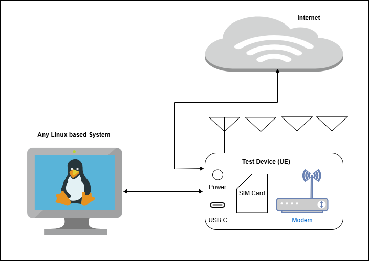
Massive MIMO and Beamforming

What is MIMO

MIMO (Multiple Input Multiple Output) antenna technology is a way of increasing the capacity of a radio link using multiple transmit antennas and multiple receive antennas. Due to multipath propagation and decorrelated paths between the transmitter and receiver, multiple data streams can be sent over the same radio channel, thus increasing the peak data rate per user along with the capacity of the cellular network. MIMO has been part of LTE since the 1st release. LTE started with a 2×2 MIMO which means 2 transmit antennas at the base station (BS) side and 2 receive antennas at the UE side. LTE allow applications of up to 8 spatial layers in DL direction and up to 4 spatial layers in UL direction. Commercial LTE networks tend to use 2 or 4 spatial layers.

MIMO can be implemented in many ways:

  • Diversity: Multiple transmit and receive antennas are used to increase coverage (increased signal to interference plus noise ratio, SINR). Transmit diversity means to have multiple antennas at the sending side and receive diversity means to have multiple antennas at the receiver side to increase the captured radio energy.
  • Spatial Multiplexing: When multiple antennas are used by both sender and receiver, multiple streams can be sent with different information for increased user data bit rate. Transmission of data uses several layers with small phase shift between the layers, enabling a receiver to decode the layers separately.
  • Beamforming (BF): Multiple transmit antennas will direct the radio energy in a narrow sector to increase the SINR and thereby increasing the coverage (or increase the bitrate to the UE at a certain distance from the BS).

If different data streams are sent to the same receiver, it is referred to as Single User MIMO (SU-MIMO), while if the data streams are transmitted to different users, it is referred to as Multi-User MIMO (MU-MIMO)

Difference between SU-MIMO and MU-MIMO

With 5G NR, there is possibility of having up to 256 transmit antenna at the BS side and that is where the term ‘massive MIMO’ comes into picture. Massive MIMO antennas uses a large number of antenna elements but operate at frequencies below 6 GHz. Essentially, they exploit many elements to realize a combination of BF and spatial multiplexing.

Beamforming (BF) Fundamentals

Beamforming is a well-known and established antenna technology. Cellular networks such as LTE apply this technology to improve overall performance. Objects are identified by radar applications using Beamforming. It has more importance in 5G cellular communications as it allows deployment of 5G in higher frequency ranges such as cm-wave and mm-wave frequency spectrum where it is necessary to achieve enough cell coverage i.e. to compensate for high path loss at these frequencies.

The ability to steer beams dynamically is equally important since blockage scenarios are likely to occur due to moving objects such as cars or even a human body which can block the line of sight path. Consider some examples below:

  • In a fixed wireless access scenario, the customer premises equipment (CPE) in a household connects to an outdoor 5G BS. Here, no mobility is involved and a beam sweeping procedure would identify the best beam to be used.
  • In contrast, Beamforming needs to be dynamic (steerable or switchable) when a moving car on a road is connected.
Beamforming Scenarios

Support for BF is an essential capability in 5G NR which impacts the physical layer and higher layer resources. It is based on 2 fundamental physical resources: SS/PBCH blocks and the capability to configure channel state information reference signals (CSI-RS).

The principle of BF is to use the large number of antennas in, for example, an array. Each antenna can be controlled with a phase shifter and an attenuator. The antennas are usually half a wavelength of the signals they are optimized for. The phase of each antenna is then adjusted in order to control the direction of the beam. Preferably, the beam should be sent in the same direction as the UE transmitted in the UL. This means that the antennas and the logic controlling them must be able to measure the so called ‘angle of arrival’. If a signal comes from a direction in front of the antenna, all elements will receive a phase front of the signal at the same time. For Example: if the angle is 45 degrees, the antennas will receive the phase front of the signal with the time spread. By measuring the time delay between the arriving phase front to the antennas, it is possible to calculate the angle of arrival. To send the signal in the same direction, the phase front of the transmitted signal should be sent with the same time spread. Phase shifting can be done in the digital domain or analog domain.

Example of Phase array feeding network for BF with time dispersion of transmitted signal

Beamforming in 5G NR should be able to direct beams not only in horizontal direction but vertical direction as well, which is sometimes referred to as 3D MIMO as well. To be able to do that, antennas need to be put in a square, termed as Uniform Square Array (USA). Below is an example of 128 cross polarized antennas:

Uniform Square Array

By having the possibility to pack antennas and radio equipment very tightly, it is now possible to create antenna solutions with integrated antennas, analog to digital converters and power amplifiers. The antennas are put in a USA with cross-polarized antennas with 32, 64 or 256 antennas. Behind the Digital-to-analog-converter (DAC) is the baseband part which creates and analyzes the signals in the digital form, which comprises of number of Digital signal processors (DSP) with high capacity.

Example of Massive MIMO Based solution

As mentioned above, by measuring the phase front of the signal arriving to different antenna elements, it is possible to measure from which direction the signal comes in (Angle or arrival). To direct the radio energy in the same direction back to the UE, the same principle is used. This means that beams will be created from the antenna in different directions. By using different combinations of antennas, different beams can be created at the same time to different UEs located in different directions. However, the number of power amplifiers behind the antennas decide how many simultaneous beams can be created by the antenna. For Example: 8 beams can be created with 8 power amplifiers. The challenge is to pack amplifiers in an antenna and to reduce/remove the heat created by them as well as to limit the disturbance they cause to each other.

As a matrix is used, it is also possible to change the direction of the radio beam in both horizontal and vertical directions. In some case, it is referred to as 3D Beam Forming. This concept of creating beams from a Base Station will be a necessity in 5G NR when operating in very high frequency bands (FR2) due to bad radio propagation properties in these bands.

Similar principle can also be used on the receiver side in the UE or in the gNB receiver. The phase array can be set to amplify a signal arriving from a certain direction, which means that the receiver can focus on its antenna in a specific direction which is also referred to as Receiver side beam forming.

Operations in Beam Management

  • Beam Measurement: UE provides measurement reports to the Base Station on a per beam basis.
  • Beam Detection: UE identifies the best beam based on power measurements related to configured thresholds.
  • Beam Recovery: UE is configured with basic information to recover a beam in case the connection is lost.
  • Beam Sweeping: Using multiple beams at the Base Station to cover a geographic area and sweep through them at prespecified intervals.
  • Beam Switching: UE switches between different beams to support mobility scenarios.

Types of Beamforming

  • Analog BF: In this implementation, the baseband signal is 1st modulated then amplified and then split among the available number of antennas. Each RF chain has the capability to change the amplitude and phase individually. Analog BF in the RF path is simple and uses a minimal amount of hardware, making it the most cost-effective way to build a BF array. The drawback is that system can only handle one data stream and generate one signal beam. The beams must be time multiplexed and beams pointing in different directions are separated in time.
  • Digital BF: In this implementation, multiple digital streams are already generated in the baseband and as before, each is individually modified in phase and amplitude to generate the desired beam. So, several sets can be created and superimposed before feeding the array elements. This mechanism enables one antenna to generate multiple beams, each with its own signal and serving multiple users. Here, phase shifting is done before the Digital to Analog Conversion. BF modifications of the signals will be made in DSP by modifying the digital representation of the signal. This is the preferred method for lower frequencies in 5G as the advantage is that the phase and amplitude of each antenna can be controlled separately giving high flexibility. If each antenna can be controlled, full flexibility is possible with the number of beams the antenna can create at the same time. Here, phase shifting is done before the Digital to Analog Conversion. BF modifications of the signals will be made in DSP by modifying the digital representation of the signal. This is the preferred method for lower frequencies in 5G as the advantage is that the phase and amplitude of each antenna can be controlled separately giving high flexibility. If each antenna can be controlled, full flexibility is possible with the number of beams the antenna can create at the same time.
Difference between Analog and Digital Beamforming
  • Hybrid BF: This implementation combines both the above-mentioned methods. A limited number of digital streams feed multiple analog beamformers, whereas each is connected to a subset of total elements in the antenna array, which provides a compromise between implementation complexity, cost and flexibility.
Difference between Analog, Hybrid and Digital Beamforming

Note: Digital BF seems to be the most obvious way to implement Spatial Multiplexing as same signal can be sent from all the antennas to a particular user, with possible variation in phase/amplitude per antenna or possible variation in phase/amplitude per subcarrier. This is particularly important for cases where there is no direct line of sight between the Base station and the user.

Evolution of Massive MIMO

It is generally acknowledged that network densification is one of the main solutions to the exploding demand for capacity. Densification, when defined as the number of antennas per unit area, can be achieved through multi‐antenna systems such as massive MIMO.

Network densification proposes the deployment of a large number of antennas per cell site, to form what is known as a ‘massive MIMO’ (multi‐user MIMO with very large antenna arrays) network, once the number of antennas exceeds the number of active UEs per cell. This emerging technology uses multiple co‐located antennas (up to a few hundred) to simultaneously serve / spatially multiplex several users in the same time‐frequency resource. As the aperture of the array grows with many antennas, the resolution of the array also increases. This effectively concentrates the transmitted power towards intended receivers, thus the transmit power can be made arbitrarily small, resulting in significant reductions in intra‐ and inter‐cell interference. Distributing antennas has also been shown to result in highest capacity.

The antennas used for the macro cells are 2×4 MIMO and those used for the small cells are 128×4 MIMO (i.e. Massive MIMO). According to DoCoMo, “the aim of using Massive MIMO is to bar jamming through the beamforming technology”.

Approach for Massive MIMO

The approach here is to base all the beams on the uplink channel estimation. Here, UE sends a pilot signal which will be a known signal and Base station estimates what it receives, and, on that basis, it estimates the channel for the users. Thus, Base station can find some well-matched estimates to the channel and there is no need to make assumptions from beginning as to how channel looks like. Base station can just measure what it sees. It is also scalable with many antennas. This approach is different from the conventional approach where different angular beams are tried and user reports the best one, which is not a very nice solution as there is possibility of a user to be at the boundary and it can cause too much inter-user interference.

If the number of applied antenna elements is significantly increased at the Base station, for example if 64 cross-polarized antennas are used, the network node becomes a massive MIMO BS. Even with the increased number of antenna elements, the number of spatial layers is not increased. 5G NR supports 8 layers on the DL and 4 layers on the UL. However, large number of antenna elements allows the combinations of beamforming with spatial multiplexing. So, Massive MIMO antennas enabled focused transmission and reception of signal energy in the smaller regions of space, which brings huge improvements in user throughput, capacity and energy efficiency, especially when combined with simultaneous scheduling of multiple users.

In the established sub-6 GHz frequency spectrum, Base Station apply a large number of TX/RX antenna elements to serve multiple users with parallel data streams with moderate antenna gains. In contrast, the high path loss attenuation in the cm-wave and mm-wave bands requires high antenna gains. Consequently, both the Base Station and UE antenna implementations focus on high gain and dynamic Beamforming algorithms i.e. all available TX elements are used to create a single beam.

Distributed MIMO

NR is ready to support distributed MIMO however the support was not complete in release 15. Distributed MIMO implies that the device can receive multiple independent physical data shared channels (PDSCHs) per slot to enable simultaneous data transmission from multiple transmission points to the same user which means that some MIMO layers are transmitted from one site while other layers are transmitted from another site.

Advantages of Massive MIMO

  • With a greater number of antennas, beam width will be smaller (Narrower Beam due to involvement of fewer multipath components) leading to higher reliability and lower latency. This essentially means that the number of lost packets would be less and hence lesser retransmissions.
  • Resource allocations are made simple in Massive MIMO. All subcarriers are good at all times. So, no need to schedule based on fading. Each user gets the whole bandwidth whenever needed.
  • Massive MIMO can be very useful with:
    • Mobile Broadband applications
      • Very high spectral efficiency, multiplex many users
      • Great improvements at the cell edge
    • Ultra-Reliable Low Latency Communication (URLLC)
      • Lesser lost packets, so Fewer retransmissions
      • more predictable performance in the networks
    • Massive Machine-Type Communication (mMTC)
      • Can extend coverage, more cost-efficient deployment by putting up fewer Base Station in order to reach all the sensors.
      • Can help reduce transmit power for battery powered devices

Limitations of Massive MIMO

  • Works only with Time Division Duplex (TDD) mode where you change between UL and DL on the same frequency and for that reason, you can measure the channel in the UL and use it also for DL transmission.
  • The performance of massive MIMO is limited by the finite and correlated scattering given the space constraints. The degrees of freedom of the system, solely determined by the spatial resolution of the antenna array, can reach saturation point. Also, in frequency division duplex (FDD) systems, channel estimation and feedback for a large number of antennas presents a challenge. Unless the channel structure is available at the BS, the prohibitive downlink channel training and feedback in FDD systems sets an upper limit on the number of BS antennas.
  • With Massive MIMO, there is a challenge of manufacturing many low cost, low-precision components which also affects how to approach testing and verification of the performance of these antennas since over the air test methods must generally be applied.

Since this was just an introduction article, I might write another one in future to cover up more details about Massive MIMO.

References

Carrier Aggregation

Introduction

Carrier Aggregation is a technology that aggregates multiple component carriers (CC), which can be jointly used for transmission to/from a single device. It combines two or more carriers into one data channel to enhance the data capacity of a network. Using existing spectrum, Carrier Aggregation helps mobile network operators (MNOs) in providing increased UL and DL data rates. When Carrier Aggregation is deployed, frame timing and SFN are aligned across cells that can be aggregated. 5G NR utilizes CA in both FR1 and FR2, supporting up to 16 component carriers. For Release 15, the maximum number of configured Component Carriers for a UE is 16 for DL and 16 for UL.

Important characteristics:

  • Up to 16 carriers (contiguous and non-contiguous) can be aggregated
  • Carriers can use different numerologies
  • Transport block mapping is per carrier
  • Cross carrier scheduling and joint feedback are also supported
  • Flexibility for network operators to deploy their licensed spectrum by using any of the CA types (such as intra-band contiguous, intra-band noncontiguous or inter-band noncontiguous)

History

LTE release 10 introduced enhanced LTE spectrum flexibility through carrier aggregation which was required to support higher bandwidths and fragmented spectra. Up to 5 component carriers, possibly each of different bandwidth, can be aggregated in this release, allowing for transmission bandwidths of up to 100MHz.  All component carriers need to have the same duplex scheme and in the case of TDD, same uplink downlink configuration.

In LTE release 10, Backwards compatibility was ensured as each component carrier uses the release-8 structure. Hence, to a release-8/9 device each component carrier will appear as an LTE release-8 carrier, while a carrier-aggregation capable device can exploit the total aggregated bandwidth, enabling higher data rates. In the general case, a different number of component carriers can be aggregated for the downlink and uplink. This was an important property from a device complexity point of view where aggregation can be supported in the downlink where very high data rates are needed without increasing the uplink complexity.

Release 13 marked the start of LTE Advanced Pro, included various enhancements in Carrier Aggregation. The number of component carriers possible to aggregate was increased to 32, resulting in a total bandwidth of 640MHz and a theoretical peak data rate around 25 Gbit/s in the DL considering 8 layers spatial multiplexing and 256 QAM. The main motivation for increasing the number of subcarriers was to allow for very large bandwidths in unlicensed spectra.

LTE release 13 also introduced license-assisted access, where the carrier aggregation framework is used to aggregate downlink carriers in unlicensed frequency bands, primarily in the 5 GHz range, with carriers in licensed frequency bands. Mobility, critical control signaling and services demanding high quality-of-service rely on carriers in the licensed spectra while (parts of) less demanding traffic can be handled by the carriers using unlicensed spectra.

In LTE release 14, license-assisted access was enhanced to address uplink transmissions also.

Carrier aggregation was one of the most successful enhancements of LTE till now with new combinations of frequency band added in every release.

Carrier Aggregation in NR

Like LTE, multiple NR carriers can be aggregated and transmitted in parallel to/from the same device, thereby allowing for an overall wider bandwidth and correspondingly higher per-link data rates. The carriers do not have to be contiguous in the frequency domain but can be dispersed, both in the same frequency band as well as in different frequency bands, resulting in three difference scenarios:

Intraband aggregation with frequency-contiguous component carriers;

Intraband aggregation with non-contiguous component carriers;

Interband aggregation with non-contiguous component carriers.

Below figure depicts these 3 scenarios:

Carrier Aggregation Types

Although the overall structure is the same for all three cases, the RF complexity can be vastly different.

Up to 16 carriers, having different bandwidths and different duplex schemes, can be aggregated allowing for overall transmission bandwidths of up to 6,400 MHz (16 x 400 MHz) = 6.4 GHz, which is more than typical spectrum allocations.

A device capable of CA may receive or transmit simultaneously on multiple component carriers while a device not capable of CA can access one of the component carriers. It is worth noting that in the case of Inter-band carrier aggregation of multiple half-duplex (TDD) carriers, the transmission direction on different carriers does not necessarily have to be the same. This implies that a carrier-aggregation-capable TDD device may need a duplex filter, unlike the typical scenario for a noncarrier-aggregation-capable device.

In the specifications, carrier aggregation is described using the term cell, that is, a carrier-aggregation-capable device can receive and transmit from/to multiple cells. One of these cells is referred to as the primary cell (PCell). This is the cell which the device initially finds and connects to, after which one or more secondary cells (SCells) can be configured, once the device is in connected mode. The secondary cells can be rapidly activated or deceived to meet the variations in the traffic pattern. Different devices may have different cells as their primary cell—that is, the configuration of the primary cell is device-specific. Furthermore, the number of carriers (or cells) does not have to be the same in UL and DL. In fact, a typical case is to have more carriers aggregated in the DL than in the UL. Reasons being:

  • There is typically more traffic in the DL that in the UL.
  • The RF complexity from multiple simultaneously active uplink carriers is typically larger than the corresponding complexity in the downlink.

Carrier aggregation uses L1/L2 control signaling for the same reason as when operating with a single carrier. As baseline, all the feedback is transmitted on the primary cell, motivated by the need to support asymmetric carrier aggregation with the number of downlink carriers supported by a device different than the number of uplink carriers. For many downlink component carriers, a single uplink carrier may carry a large number of acknowledgments. To avoid overloading a single carrier, it is possible to configure two PUCCH groups where feedback relating to the first group is transmitted in the uplink of the PCell and feedback relating to the other group of carriers is transmitted on the primary second cell (PSCell).

Multiple PUCCH Groups

If carrier aggregation is used, the device may receive and transmit on multiple carriers, but reception on multiple carriers is typically only needed for the highest data rates. It is therefore beneficial to inactivate reception of carriers not used while keeping the configuration intact. Activation and inactivation of component carriers can be done through MAC signaling containing a bitmap where each bit indicates whether a configured SCell should be activated or deactivated.

Difference between self-scheduling and cross-carrier scheduling

Scheduling grants and scheduling assignments can be transmitted on either the same cell as the corresponding data, known as self-scheduling, or on a different cell than the corresponding data, known as cross-carrier scheduling.

Self-scheduling vs Cross-scheduling

Let’s discuss in detail – the scheduling decisions are taken per carrier and the scheduling assignments are transmitted separately for each carrier, that is, a device scheduled to receive data from multiple carriers simultaneously receives multiple PDCCHs. A PDCCH received can either point to the same carrier, known as self-scheduling, or to another carrier, commonly referred to as cross-carrier scheduling or cross-scheduling. In case of cross-carrier scheduling of a carrier with a different numerology than the one upon which the PDCCH was transmitted, timing offsets in the scheduling assignment, for example, which slot the assignment relates to, are interpreted in the PDSCH numerology (and not the PDCCH numerology).

Carrier Aggregation support in MAC Layer

MAC Layer is responsible for multiplexing/demultiplexing data across multiple component carriers when carrier aggregation is used. In case of CA, it is responsible for distributing data from each flow across the different component carriers, or cells.

The basic principle for carrier aggregation is independent processing of the component carriers in the physical layer, including control signaling, scheduling and HARQ retransmissions, while carrier aggregation is invisible above the MAC layer. Carrier aggregation is therefore mainly seen in the MAC layer, where logical channels, including any MAC control elements, are multiplexed to form transport blocks per component carrier with each component carrier having its own HARQ entity.

Carrier Aggregation in MAC

Note: In the case of carrier aggregation, there is one DL-SCH (or UL-SCH) per component carrier seen by the device

Relation with Dual Connectivity

Dual connectivity implies that a device is simultaneously connected to two cells. User-plane aggregation, where the device is receiving data transmission from multiple sites, separation of control and user planes, and uplink-downlink separation where downlink transmissions originate from a different node than the uplink reception node are some examples of the benefits with dual connectivity. To some extent it can be seen as carrier aggregation extended to the case of non-ideal backhaul. It is also essential for NR when operating in non-standalone mode with LTE providing mobility and initial access.

Example of Dual Connectivity

In dual connectivity, a device is connected to two cells, or in general, two cell groups, the Master Cell Group (MCG) and the Secondary Cell Group (SCG). The reason for the term cell group is to cover also the case of carrier aggregation where there are multiple cells, one per aggregated carriers, in each cell group. The two cell groups can be handled by different gNBs.

Dual Connectivity Details

A radio bearer is typically handled by one of the cell groups, but there is also the possibility for split bearers, in which case one radio bearer is handled by both cell groups. In this case, PDCP is in charge of distributing the data between the MCG and the SCG and thus PDCP plays an important role for Dual connectivity support.

Differences between Dual Connectivity and Carrier Aggregation

Both carrier aggregation and dual connectivity result in the device being connected to more than one cell. Despite this similarity, there are fundamental differences, primarily related to how tightly the different cells are coordinated and whether they reside in the same or in different gNBs.

Carrier aggregation implies very tight coordination, with all the cells belonging to the same gNB. Scheduling decisions are taken jointly for all the cells the device is connected to by one joint scheduler. Dual connectivity, on the other hand, allows for a much looser coordination between the cells. The cells can belong to different gNBs, and they may even belong to different radio-access technologies as is the case for NR-LTE dual connectivity in case of non-standalone operation.

Carrier aggregation and dual connectivity can also be combined. This is the reason for the terms master cell group and secondary cell group. Within each of the cell groups, carrier aggregation can be used.

Multi Connectivity includes Dual Connectivity (PDCP UP Split) and Carrier Aggregation (MAC UP Split) as shown in the figure below:

Carrier Aggregation with Dual Connectivity

Dual Connectivity should be preferred when latency is not neglectable between paths i.e. > 5-10ms or when there is a different RAT to be connected and TN of the master side is congested, whereas Carrier Aggregation has better and faster utilization of radio resources than Dual Connectivity but is used to connect same RATs. It requires low inter site latency (<5ms).

Note:

  • In the case of carrier aggregation or dual connectivity, multiple power headroom reports can be contained in a single message (MAC control element).
  • NR does not support carrier aggregation with LTE and thus dual connectivity is needed to support aggregation of the LTE and NR throughput.
  • NR specifications supports carrier aggregation, where multiple carriers are present within a band, or in multiple bands, can be combined to create larger transmission bandwidths.

Relation with Supplementary Uplink

Both these techniques allow the uplink transmission to be switched between the FDD-band and the 3.5 GHz band. The use of these mechanisms effectively utilizes idle sub-3 GHz band resources, improve the uplink coverage of C-band, and enable the provisioning of 5G services in a wider area. Both solutions, NR Carrier Aggregation and Supplementary Uplink, offer transport of UL user data using sub-3GHz band NR radio resources. NR CA provides the added benefit of also providing sub-3GHz DL user data support on the FDD-band downlink, using 3GPP specified LTE-NR spectrum sharing, if needed. This provides opportunity to aggregate NR bandwidth as well as better operation of the NR uplink.

Difference between Carrier Aggregation (CA) and supplementary uplink (SUL)

Supplementary uplink differs from the aggregated uplink in that the UE may be scheduled to transmit either on the supplementary uplink or on the uplink of the carrier being supplemented, but not on both at the same time.

In a typical carrier aggregation scenario:

  • Main aim of carrier aggregation is to enable higher peak data rates by increasing the bandwidth available for transmission to/from a device.
  • The two (or more) carriers are often of similar bandwidth and operating at similar carrier frequencies, making aggregation of the throughput of the two carriers more beneficial. Each uplink carrier is operating with its own associated downlink carrier, simplifying the support for simultaneous scheduling of multiple uplink transmissions in parallel. Formally, each such downlink carrier corresponds to a cell of its own and thus different uplink carriers in a carrier-aggregation scenario correspond to different cells.

While in case of SUL scenario:

  • Main aim of SUL is to extend uplink coverage, that is, to provide higher uplink data rates in power-limited situations, by utilizing the lower path loss at lower frequencies
  • The supplementary uplink carrier does not have an associated downlink carrier of its own. Rather, the supplementary carrier and the conventional uplink carrier share the same downlink carrier.  Consequently, the supplementary uplink carrier does not correspond to a cell of its own. Instead, in the SUL scenario there is a single cell with one downlink carrier and two uplink carriers.
Carrier Aggregation vs Supplementary Uplink

Benefits of Carrier Aggregation

  • Better Network Performance: Carriers provide a more reliable and stronger service with less strain on individual networks.
  • Leveraging of underutilized spectrum: CA enables carriers to take advantage of underutilized and unlicensed spectrum, thereby extending the benefits of 5G NR to these bands.
  • Increased uplink and downlink data rates: Wider bandwidth mean higher data rates.
  • More efficient use of spectrum: Operators can combine fragmented smaller spectrum holdings into larger and more useful blocks and can create aggregated bandwidths greater than those that would be possible from a single component carrier.
  • Network carrier load balancing: Enables intelligent and dynamic load balancing with real‐time network load data.
  • Higher capacity: CA doubles the data rate for users while reducing latency with a good amount.
  • Scalability: Expanded coverage allows carriers to scale their networks rapidly.
  • Dynamic switching: CA enables dynamic flow switching across component carriers (CCs).
  • Better user experience: CA delivers a better user experience with higher peak data rates (particularly at cell edges), higher user data rates, and lower latency, as well as more capacity for “bursty” usage such as web browsing and streaming video.
  • Enabling of new mobile services: Delivering a better user experience opens opportunities for carriers to innovate and offer new high bandwidth/high data rate mobile services.
  • Can be combined with Dual Connectivity

Disadvantages/Challenges with Carrier Aggregation:

  • Intra‐band uplink CA signals use more bandwidth and have higher peak‐to‐average power ratios (PAPRs)
  • Many possible configurations of resource blocks (RBs) exist in multiple component carriers (CCs) where signals could mix and create spurious out‐of‐band problems.
  • Intra‐band CA signals present mobile device designers with many challenges because they can have higher peaks, more signal bandwidth, and new RB configurations. A Power Amplifier design must be tuned for very high linearity even though the signal power may be backed off. Adjacent channel leakage, intermodulation products of non‐contiguous RBs, spurious emissions, noise, and sensitivity must be considered. The tradeoff of linearity comes at the expense of efficiency and thermal effects.
  • Inter‐band CA combines transmit signals from different bands. The maximum total power transmitted from a mobile device is not increased in these cases, so for two transmit bands, each band carries half the power of a normal transmission, or 3 dB less than a non‐CA signal. Because different PAs are used to amplify the signals in different bands, and the transmit power is reduced for each, the PA linearity isn’t an issue. Other front‐end components, like switches, have to deal with high‐level signals from different bands that can mix and create intermodulation products. These new signals can interfere with one of the active cellular receivers or even another receiver on the phone, like the GPS receiver. To manage these signals, switches must have very high linearity.

References:

  1. https://www.gsma.com/futurenetworks/wp-content/uploads/2019/03/5G-Implementation-Guideline-v2.0-July-2019.pdf
  2. “5G NR – The next generation wireless access technology” – By Erik Dahlman, Stefan Parkvall, Johan Sköld
  3. https://www.3gpp.org/technologies/keywords-acronyms/101-carrier-aggregation-explained
  4. https://www.qorvo.com/design-hub/ebooks/5g-rf-for-dummies

HARQ

Introduction

5G NR (New radio) has several retransmission systems using three different layers in the protocol stack:

  • MAC protocol: It implements a fast retransmission system with delay less than 1ms in new radio, called HARQ (Hybrid Automatic Repeat reQuest).
  • RLC protocol: Even though HARQ is present at MAC but there might still be some possibility of errors in the feedback system. So, for dealing with those errors, RLC has a slow retransmission system but with a feedback protected by CRC. Compared to the HARQ acknowledgments, the RLC status reports are transmitted relatively infrequently.
  • PDCP protocol: This will guarantee in-sequence delivery of user data and it is mainly used during handover as RLC and MAC buffers are flushed when a handover is executed.

NR uses an asynchronous hybrid-ARQ protocol in both downlink and uplink, that is, the hybrid-ARQ process which the downlink or uplink transmission relates to is explicitly signaled as part of the downlink control information (DCI). The hybrid-ARQ mechanism in the MAC layer targets very fast retransmissions and, consequently, feedback on success or failure of the downlink transmission is provided to the gNB after each received transport block (for uplink transmission no explicit feedback needs to be transmitted as the receiver and scheduler are in the same node).

HARQ is implemented to correct the erroneous packets coming from PHY layer. If the received data is erroneous then the receiver buffers the data and requests for a re-transmission from the sender. When the receiver receives the re-transmitted data, it then combines it with buffered data prior to channel decoding and error detection. This helps in the performance of re-transmissions. For this to work, the sending entity need to buffer the transmitted data until the ACK is received since the data needs to be retransmitted in case a NACK is received.

HARQ is a stop and wait (SAW) protocol with multiple processes. The protocol will continue to repair one transmission without hindering other ongoing transmissions which can continue in parallel.

HARQ principle with multiple processes

Why multiple SAW processes are required?

Once a packet is sent from a process, it waits for an ACK/NACK. While it is waiting for an ACK/NACK in the active state, no other work can be done by the same process leading to reduced performance. So, if we have multiple such processes working in parallel, throughput can be increased by making other processes work at the same time on other packets, while a process is in waiting state for ACK/NACK.

Differences with LTE HARQ

  • New radio is using an asynchronous protocol in both UL and DL, which is different from LTE, where the protocol was synchronous in UL; UE should reply with an ACK/NACK after 3ms of receiving the DL data. The gNB knows that when the ACK/NACK is expected. In NR, the report timing is not fixed to increase the flexibility which is important for URLLC services.
  • PHICH (Physical HARQ Indicator channel) was used in LTE to handle uplink retransmissions and was tightly coupled to the use of a synchronous HARQ protocol, but since the NR HARQ protocol is asynchronous in both uplink and downlink the PHICH is not needed in NR.
  • In LTE, Non-adaptive retransmissions were triggered by a negative acknowledgement on the PHICH, which used the same set of resources as the previous transmission i.e. the modulation scheme and the set of allocated resource blocks remains unchanged. Only Redundancy version used to change between transmissions. But in NR, PHICH is not there and retransmissions are adaptive that can be triggered by DCI. NDI flag retriggers a transmission if its value is toggled relative to previous transmission.
  • Maximum number of HARQ processes was set to 8 in LTE but is increased to 16 in NR. This was motivated by shorter time slot and increased use of remote radio heads that will increase the round-trip time slightly.

Reasons why NR HARQ is asynchronous in both UL and DL:

  • Synchronous HARQ operation does not allow dynamic TDD.
  • Operation in unlicensed spectra (part of later NR releases) is more efficient with asynchronous operation as it is not guaranteed that the radio resources are available at the time for a synchronous transmission.

Hybrid ARQ with Soft combining

The hybrid-ARQ protocol is the primary way of handling retransmissions in NR. In case of an erroneously received packet, a retransmission is requested. However, despite it not being possible to decode the packet, the received signal still contains information, which is lost by discarding erroneously received packets. This shortcoming is addressed by hybrid-ARQ with soft combining. In hybrid- ARQ with soft combining, the erroneously received packet is stored in a buffer memory and later combined with the retransmission to obtain a single, combined packet that is more reliable than its constituents. Decoding of the error-correction code operates on the combined signal. Both Chase combining and Incremental Redundancy methods were proposed initially, but it is Incremental Redundancy that is getting used in NR.

Difference between Chase combining and Incremental Redundancy

In Chase combining, the physical layer applies the same puncturing pattern to both the original transmission and each retransmission. This results in retransmissions which include the same set of physical layer bits as the original transmission. Systematic bit remains the same even in the subsequent transmission. Only Parity 1 and Parity 2 bits are punctured. Benefits of chase combining are its simplicity and lower UE memory requirements.

Example of Chase Combining

In Incremental Redundancy, the physical layer applies different puncturing patterns to the original transmission and retransmission. This results in retransmission which include a different set of physical layer bits to the original transmission. 1st transmission provides the systematic bits with the greatest priority while subsequent retransmissions can provide either the systematic or the parity 1 and parity 2 bits with greatest priority. Drawbacks associated with Incremental Redundancy are its increased complexity and increased UE memory requirements.

Example of Incremental redundancy

Performance wise, incremental redundancy is like chase combining when the coding rate is low i.e. there is less puncturing. But, when there is an increased quantity of puncturing, the performance of incremental redundancy becomes greater i.e. when the coding rate is high because channel coding gain is greater than soft combining gain.

Codeblock Groups

Due to increased data rate in NR, when several gigabits per second is transmitted, the size of the transport block will be too large to handle. So, these transport blocks will be split into codeblocks, each with its own 24 bits CRC. This principle made it possible to handle large transport block in parallel channel coders/decoders.

In NR, there can be hundreds of codeblocks in a transport block. If only one or a few of them are in error, retransmitting the whole transport block results in a low spectral efficiency compared to retransmitting only the erroneous codeblocks.

To reduce the control signaling overhead, 2,4,6 or 8 blocks can be grouped together to Codeblock Groups (CBG). In case of an error in one Codeblock, only the Codeblock group to which the faulty Codeblock belongs, need to be retransmitted instead of whole transport block. If per-Code Block Group (per-CBG) retransmission is configured, feedback is provided per CBG instead of per transport block and only the erroneously received codeblock groups are retransmitted, which consumes less resources than retransmitting the whole transport block.

Retransmission of single Codeblock group

HARQ in Downlink

The gNB will send a scheduling message to the UE that indicates where the user data is located and how it is coded. Downlink Control Information (DCI) will indicate which HARQ process to be used by the UE. Since transmissions and retransmissions are scheduled using the same framework, the UE needs to know whether the transmission is a new transmission, in which case the soft buffer should be flushed, or a retransmission, in which case soft combining should be performed. For that purpose, a New Data Indicator (NDI) bit will also be set to indicate that this will be new data and the receive buffer should be flushed before loading the user data.

Upon reception of a downlink scheduling assignment, UE checks the new-data indicator to determine whether the current transmission should be soft combined with the received data currently in the soft buffer for the HARQ process in question, or if the soft buffer should be cleared. UE receives the user data and starts to calculate a checksum of the single transport block and if used, the included codeblocks. After completing the calculation, the UE follows the timing order of the UL report and sends an HARQ report indicating ACK or NACK. In case of NACK, the gNB will start to schedule a retransmission of the data.

HARQ in Downlink
Retransmission of code block in DL

Now if per- CBG retransmissions are configured, UE needs to know which CBGs are retransmitted and whether the corresponding soft buffer should be flushed or not. For this purpose, two additional fields are present in the DCI. 1) CBG Transmit Indicator (CBGTI), which is a bitmap indicating whether a certain CBG is present in the downlink transmission or not and 2) CBGFI which is a single bit, indicating whether the CBGs indicated by the CBGTI should be flushed or whether soft combining should be performed.

Example of per-CBG retransmission

The result of the decoding operation—a positive acknowledgment in the case of a successful decoding and a negative acknowledgment in the case of unsuccessful decoding—is fed back to the gNB as part of the uplink control information. If CBG retransmissions are configured, a bitmap with one bit per CBG is fed back instead of a single bit representing the whole transport block.

DCI Format 1-0 and 1-1 for downlink scheduling assignment contains HARQ related information as:

  • Hybrid-ARQ process number (4 bit), informing the device about the hybrid-ARQ process to use for soft combining.
  • Downlink assignment index (DAI, 0, 2, or 4 bit), only present in the case of a dynamic hybrid-ARQ codebook. DCI format 1_1 supports 0, 2, or 4 bits, while DCI format 1_0 uses 2 bits.
  • HARQ feedback timing (3 bit), providing information on when the hybrid- ARQ acknowledgment should be transmitted relative to the reception of the PDSCH.
  • CBG transmission indicator (CBGTI, 0, 2, 4, 6, or 8 bit), indicating the code block groups. Only present in DCI format 1_1 and only if CBG retransmissions are configured.
  • CBG flush information (CBGFI, 0_1 bit), indicating soft buffer flushing. Only present in DCI format 1_1 and only if CBG retransmissions are configured.

HARQ in Uplink

The gNB sends a scheduling message to the UE indicating resources to be used for uplink transmission, which also has HARQ process number. The UE will follow the order and send the transport block (or Codeblock group) as per the scheduling grant. The gNB will calculate and verify the checksum for the correctness of the message. The gNB will order the UE to retransmit the transport block again with a new scheduling grant, if an error id detected. In order to indicate a retransmission is required, same HARQ process number is sent with NDI bit set to no, which will be interpreted by the UE as retransmission.     

HARQ in UL
Retransmission of a transport block in UL

The CBGTI is used in a similar way as in the downlink to indicate the codeblock groups to retransmit in the case of per-CBG retransmission. Note that no CBGFI is needed in the uplink as the soft buffer is located in the gNB which can decide whether to flush the buffer or not, based on the scheduling decisions.

DCI format 0-0 and 0-1 for uplink scheduling grants also contains HARQ related information as:

  • Hybrid ARQ process number (4 bit), informing the device about the hybrid-ARQ process to (re)transmit.
  • Downlink assignment index (DAI), used for handling of hybrid-ARQ codebooks in case of UCI transmitted on PUSCH. Not present in DCI format 0_0.
  • CBG transmission indicator (CBGTI, 0, 2, 4, or 6 bit), indicating the code block groups to retransmit. Only present in DCI format 0_1 and only if CBG retransmissions are configured.

Timing of UL reports

The timing of the UL HARQ reports was fixed in LTE as 3ms, which was way too much for 5G and URLLC services. The solution in NR is to have a flexible solution that can be modified between different service requirements and when new HW is developed. The gNB informs the UE about the timing in a ‘HARQ timing’ field in the Downlink Control Information (DCI). This flexibility was also required in dynamic TDD when the directions of the slots is flexible (UL/DL). The “HARQ Timing” field contains a 3-bit pointer to an RRC Configured Table, which will indicate the timing between the scheduling message (The data this is included in the slot) and the related UL report. This will also allow for the gNB to order several transmissions to be grouped together or to order the UE to report as quickly as possible (for delay sensitive services). This information provides the UE with the information when to send the HARQ report back to the gNB.

Now where in the frequency band the information should be sent (Physical Uplink Control Channel, PUCCH)? The answer is that RRC protocol configures another table and the UE will get a pointer to the table in the scheduling message. This will tell the UE where to send the HARQ report.

Multiple Bits in HARQ reports

5G NR supports very high bitrates and multiple simultaneous carriers. A UE can be configured to use carrier aggregation, spatial multiplexing and dual connectivity at the same time. This means that UE should be able to report the success or failure of the transmission of multiple transport blocks at the same time. To do this, there are two ways defined in the standard:

  • Semi-static HARQ acknowledgement codebook

Below example can be considered to understand semi-static HARQ acknowledgement codebook:

Example of semi-static HARQ Codebook

The codebook which is configured by RRC protocol is valid for a specific time span. In the example, it is valid for 3 slots. The upper carrier is configured to use 4 codeblocks per transport block, the middle carrier uses spatial multiplexing with either one or two transport blocks per slot. Finally, the lower carrier is using transmission with 1 transport block per slot. A configured table is shown below the figure where A/N means Ack/Nack is transmitted while only N means NACK is sent. Negative acknowledgements are always sent for Non-scheduled slots which will help the gNB to detect that a scheduling message was not received by the UE. When the UE reports, there will always be 21 bits in the report as there are 7 rows in the table and 3 slots.

  • Dynamic HARQ acknowledgement codebook

As you can see above, the drawback with semi-static codebook was that the number of bits can be rather high in case of, for example carrier aggregation with large number of component carriers. This is the reason 3GPP adopted dynamic HARQ codebook as default approach of reporting. The principle is to only report those transport blocks or codeblock groups that are actually sent, which will reduce the overhead in the reporting. However, there is a problem with this reporting method as the scheduling message sent to the UE may be lost on one of the carriers (or many carriers). This might create a situation where gNB and the UE do not agree on how many transport blocks to report. To avoid this situation, the scheduling message will indicate how many transport blocks or codeblock groups to report.

Example of dynamic HARQ Codebook

In the above example, there are 5 carrier in the carrier aggregation scenario. For every scheduling message sent on each carrier, the “cDAI” tells the number of transport block (Counter Downlink Assignment). For detecting lost scheduling messages, the total number of scheduled carriers is also indicated as “tDAI” (Total Downlink Assignment). The figure shows that the number 3, sent on carrier #3, gets lost and is not detected/decoded by the UE. This will be detected easily by the UE as the total DAI indicates that the last number should be 6 but the UE has only received number 0 to 5. The HARQ report in this case will consist of 12 bits, one for each received transport block during the time span of the codebook.

Note: To know more, Please refer to http://www.sharetechnote.com/html/5G/5G_HARQ.html

References:

Supplementary Uplink

Introduction

In 5G NR, a downlink carrier may be associated with two uplink carriers (the non-SUL carrier and the SUL carrier), where the Supplementary Uplink (SUL) carrier is typically located in lower frequency bands, thereby providing enhanced uplink coverage.

Example of Supplementary Uplink: With SUL, the UE is configured with 2 ULs for one DL of the same cell as depicted in figure below:

Example of Supplementary Uplink

Below are the Operating Bands defined by 3GPP for NR in Frequency Range 1 where the duplex mode is SUL:

Operating Bands supporting SUL as duplex mode

Supplementary Uplink (in detail)

In conjunction with a UL/DL carrier pair (FDD band) or a bidirectional carrier (TDD band), a UE may be configured with additional, Supplementary Uplink (SUL) which can improve UL coverage for high frequency scenarios.

Since the lower frequency bands are already occupied by LTE primarily, so for enabling early NR deployment in lower-frequency spectra, LTE/NR spectrum co-existence is thought of as the way for an operator to deploy NR in the same spectrum as an already existing LTE deployment. Two co-existence scenarios were identified in 3GPP and guided the NR design:

  1. LTE/NR co-existence in both DL and UL directions
  2. There is co-existence only in the UL direction, typically within the UL part of a lower-frequency paired spectrum, with NR downlink transmission taking place in the spectrum dedicated to NR, typically at higher frequencies. NR supports a supplementary uplink (SUL) to specifically handle this scenario.

SUL implies that a conventional downlink/ uplink (DL/UL) carrier pair has an associated or supplementary uplink carrier with the SUL carrier typically operating in lower-frequency bands. As an example, a downlink/uplink carrier pair operating in the 3.5 GHz band could be complemented with a supplementary uplink carrier in the 800 MHz band.

In SUL scenario, the non-SUL uplink carrier is typically significantly more wideband compared to the SUL carrier. Thus, under good channel conditions such as the device located relatively close to the cell site, the non-SUL carrier typically allows for substantially higher data rates compared to the SUL carrier. At the same time, under bad channel conditions, for example, at the cell edge, a lower-frequency SUL carrier typically allows for significantly higher data rates compared to the non-SUL carrier, due to the assumed lower path loss at lower frequencies.

In case of Supplementary Uplink, the UE is configured with 2 UL carriers for one DL carrier of the same cell, and uplink transmissions on those two UL carriers are controlled by the network to avoid overlapping PUSCH/PUCCH transmissions in time. Overlapping transmissions on PUSCH are avoided through scheduling while overlapping transmissions on PUCCH are avoided through configuration (PUCCH can only be configured for only one of the 2 ULs of the cell). In addition, initial access is supported in each of the uplink

Note:

  1. In paired spectrum, DL and UL can switch BWP independently. In unpaired spectrum, DL and UL switch BWP simultaneously. Switching between configured BWPs happens by means of RRC signaling, DCI, inactivity timer or upon initiation of random access. When an inactivity timer is configured for a serving cell, the expiry of the inactivity timer associated to that cell switches the active BWP to a default BWP configured by the network. There can be at most one active BWP per cell, except when the serving cell is configured with SUL, in which case there can be at most one on each UL carrier.
  2. When SUL is configured, a configured uplink grant can only be signaled for one of the 2 ULs of the cell
  3. SUL differs from the aggregated uplink in that the UE may be scheduled to transmit either on the supplementary uplink or on the uplink of the carrier being supplemented, but not on both at the same time.

Random Access in case of Supplementary Uplink (SUL)

For random access in a cell configured with SUL, the network can explicitly signal which carrier to use (UL or SUL). Otherwise, the UE selects the SUL carrier if and only if the measured quality of the DL is lower than a broadcast threshold. Once started, all uplink transmissions of the random-access procedure remain on the selected carrier.

SIB1 ::= SEQUENCE {

    servingCellConfigCommon  ServingCellConfigCommonSIB    OPTIONAL,   — Need R

}

ServingCellConfigCommonSIB ::= SEQUENCE {

    supplementaryUplink  UplinkConfigCommonSIB   OPTIONAL,   — Need R

}

Supplementary Uplink related configuration is present as a part of SIB1. Before initially accessing a cell, a device will thus know if the cell to be accessed is SUL cell or not. If the cell is SUL cell and the device supports SUL operation for the given band combination, initial random access may be carried out using either the SUL carrier or the non-SUL uplink carrier. The cell system information provides separate RACH configurations for the SUL carrier and the non-SUL carrier and a device capable of SUL determines what carrier to use for the random access by comparing the measured RSRP of the selected SS block with a carrier-selection threshold also provided as part of the cell system information.

  • If the RSRP is above the threshold, random access is carried out on the non- SUL carrier.
  • If the RSRP is below the threshold, random access is carried out on the SUL carrier.

In practice, the SUL carrier is thus selected by devices with a (downlink) pathloss to the cell that is larger than a certain value. The device carrying out a random-access transmission will transmit the random-access message 3 on the same carrier as used for the preamble transmission.

For other scenarios, when a device may do a random access, that is, for devices in connected mode, the device can be explicitly configured to use either the SUL carrier or the non-SUL carrier for the uplink random-access transmissions.

Control Signaling in case of Supplementary Uplink (SUL)

In the case of supplementary uplink operation, a device is explicitly configured (by means of RRC signaling) to transmit PUCCH on either the SUL carrier or on the conventional (non-SUL) carrier.

In terms of PUSCH transmission, the device can be configured to transmit PUSCH on the same carrier as PUCCH. Alternatively, a device configured for SUL operation can be configured for dynamic selection between the SUL carrier or the non-SUL carrier. In the latter case, the uplink scheduling grant will include SUL/non-SUL indicator that indicates on what carrier the scheduled PUSCH transmission should be carried. Thus, in the case of supplementary uplink, a device will never transmit PUSCH simultaneously on both the SUL carrier and on the non-SUL carrier.

If a device is to transmit UCI on PUCCH during a time interval that overlaps with a scheduled PUSCH transmission on the same carrier, the device instead multiplexes the UCI onto PUSCH. The same rule is true for the SUL scenario, that is, there is not simultaneous PUSCH and PUCCH transmission even on different carriers. Rather, if a device is to transmit UCI on PUCCH one carrier (SUL or non-SUL) during a time interval that overlaps with a scheduled PUSCH transmission on either carrier (SUL or non-SUL), the device instead multiplexes the UCI onto the PUSCH.

SUL Carrier Co-Existence with LTE UL Carrier leading to enhanced User Experience

As mentioned above, One SUL scenario is when the SUL carrier is located in the uplink part of paired spectrum already used by LTE. In other words, the SUL carrier exists in an LTE/NR uplink coexistence scenario. In many LTE deployments, the uplink traffic is significantly less than the corresponding downlink traffic. Consequently, in many deployments, the uplink part of paired spectra is not fully utilized. Deploying an NR supplementary uplink carrier on top of the LTE uplink carrier in such a spectrum is a way to enhance the NR user experience with limited impact on the LTE network.

SUL carrier coexisting with LTE Uplink Carrier

Reduction in Latency

In the case of TDD, the separation of uplink and downlink in the time domain may impose restrictions on when uplink data can be transmitted. By combining the TDD carrier with a supplementary carrier in paired spectra, latency-critical data can be transmitted on the supplementary uplink immediately without being restricted by the uplink-downlink partitioning on the normal carrier.

Difference between Carrier Aggregation (CA) and supplementary uplink (SUL)

In a typical carrier aggregation scenario:

  • Main aim of carrier aggregation is to enable higher peak data rates by increasing the bandwidth available for transmission to/from a device.
  • The two (or more) carriers are often of similar bandwidth and operating at similar carrier frequencies, making aggregation of the throughput of the two carriers more beneficial. Each uplink carrier is operating with its own associated downlink carrier, simplifying the support for simultaneous scheduling of multiple uplink transmissions in parallel. Formally, each such downlink carrier corresponds to a cell of its own and thus different uplink carriers in a carrier-aggregation scenario correspond to different cells.

While in case of SUL scenario:

  • Main aim of SUL is to extend uplink coverage, that is, to provide higher uplink data rates in power-limited situations, by utilizing the lower path loss at lower frequencies
  • The supplementary uplink carrier does not have an associated downlink carrier of its own. Rather, the supplementary carrier and the conventional uplink carrier share the same downlink carrier. Consequently, the supplementary uplink carrier does not correspond to a cell of its own. Instead, in the SUL scenario there is a single cell with one downlink carrier and two uplink carriers.
Carrier Aggregation vs Supplementary Uplink

Is there something possible like Supplementary Downlink also?

Yes, since the carrier aggregation framework allows for the number of downlink carriers to be larger than the number of uplink carriers, some of the downlink carriers can be thought of as supplementary downlinks. One common scenario is to deploy an additional downlink carrier in unpaired spectra and aggregate it with a carrier in paired spectra to increase capacity and data rates. No additional mechanisms beyond carrier aggregation are needed and hence the term supplementary downlink is mainly used from a spectrum point of view.

Is it possible to have combination of SUL Carrier and Carrier Aggregation?

In principle, it is possible to have a combination of SUL carrier and carrier aggregation, for example, a situation with carrier aggregation between two cells (two DL/UL carrier pairs) where one of the cells is SUL cell with an additional supplementary uplink carrier. However, currently there are no band combinations defined for such carrier-aggregation/SUL combinations

References:

  1. 3GPP TS 38.300 version 15.9.0 Release 15
  2. www.sharetechnote.com
  3. “5G NR – The next generation wireless access technology” – By Erik Dahlman, Stefan Parkvall, Johan Sköld

30 Important differences between 5G NR and LTE

This is my 1st blog where i will be sharing some basic differences between 5G NR and LTE. There can be multiple other differences also but these are some of the selected ones, which i wanted to share with everyone. I might add few more later. Also, i will try to elaborate more about individual difference with images and figures in my subsequent blogs, where i will be elaborating more about individual topics.

I hope that i have assembled good enough differences for basic understanding, including some protocol level differences too. Please go ahead, read them and do share your review comments or suggestions.

Happy reading !!

Always – on signal support

LTE (Long Term Evolution): was designed to support always on signals be it any condition or situation, leading to a lot of wastage of resources and required continuous evaluation. For Example: System information broadcast, signals for detection of base station, reference signals for channel estimation etc.

NR (New Radio): Always-on transmissions are minimized in order to enable higher network energy performance and higher achievable data rates, causing reduced interference to other cells.

Assigned spectrum

LTE: Just introduced support for licensed spectra at 3.5 GHz and unlicensed spectra at 5 GHz.

NR: It’s first release supports licensed-spectrum operation from below 1 GHz up to 52.6 GHz and planning is ongoing for extension to unlicensed spectra.

Flexibility support for time/frequency resources

LTE: has majorly supported fix timing/frequency for transmission in certain situations. For Ex: Uplink Synchronous HARQ protocol, where a retransmission occurs at a fixed point in time after the initial transmission.

NR: believes in configurable time/frequency resources. It avoids having transmission on fixed resources.

Channel estimation

LTE: dependent on cell-specific reference signals for channel estimation, which are always transmitted.

NR: For channel estimation, NR doesn’t include cell-specific reference signals, instead relies on user specific demodulation reference signals, which are not transmitted unless there is data to transmit, thereby improving energy performance of the network.

Dynamic uplink downlink allocation

LTE: Uplink and downlink allocation does not change over time. Even though a later feature called eIMTA allowed some dynamics in UL DL allocation.

NR: Supports dynamic TDD, which means dynamic assignment and reassignment of time domain resources between UL and DL directions.

Device and Network Processing time

LTE: Better than 3G but not enough considering future requirements under highly dense environment for certain applications

NR: Processing times are much shorter in NR for both device and network. For Example: A device must respond with an HARQ ACK within a slot or even lesser (depending on device capabilities) after receiving a downlink data transmission.

Low Latency Support

LTE: Requires MAC and RLC layers to know the amount to data to transmit before any processing takes place, which makes it difficult to support very low latency.

NR: This is one of the most important characteristics of NR. Let me explain this support by giving 2 examples below:

  1. Header structures in MAC and RLC have been chosen to enable processing without knowing the amount of data to transmit, which is especially important in the UL direction as the device may only have a few OFDM symbols after receiving the UL grant until the transmission should take place.
  2. By locating the reference signals and downlink control signaling carrying scheduling information at the beginning of transmission and not using time domain interleaving across OFDM symbols, a device can start processing the received data immediately without prior buffering, thereby minimizing the decoding delay.

Error Correcting Codes

LTE: uses Turbo coding for data, which are the best solution at the lower code rate (For example: 1/6, 1/3, 1/2)

NR: uses LDPC (Low density Parity check) coding in order to support higher data rate as it offers lower complexity at higher coding rates as compared to LTE. They perform better at higher code rates (For Example: 3/4, 5/6, 7/8)

Time Frequency Structure of Downlink control channels

LTE: Less flexible as it needs full carrier bandwidth

NR: Has more flexible time frequency structure of downlink control channels where PDCCH’s are transmitted in one or more control resource sets (CORESETS) which can be configured to occupy only part of the carrier bandwidth.

Service Data Application Protocol layer

LTE: Not present

NR: Introduced to handle new Quality of service requirements when connecting to 5G core network. SDAP is responsible for mapping QoS bearers to radio bearers according to their quality-of-service requirements.

RRC States

LTE: Supported only 2 states: Idle and Connected

NR: Supports a 3rd state also called the RRC_INACTIVE, which is introduced to reduce the signaling load and the associated delay in moving from idle-to-active transition. In this state, RRC context is kept in both the device and the gNB.

In Sequence Delivery of RLC Packets

LTE: Supports reordering and in sequence delivery of RLC PDUs to higher protocol layers, leading to more delays.

NR: doesn’t support in-sequence delivery of RLC PDUs in order to reduce the associated delay incurred by the reordering mechanism which might be unfavorable for services that require very low latency. By doing this, RLC reduces the overall latency as packets do not have to wait for retransmission of an earlier missing packet before it is delivered to higher layers but can be forwarded immediately.

Concatenation of RLC PDUs

LTE: supported it to disallow RLC PDUs to be assembled in advance

NR: Removed this from RLC protocol to support assembly of RLC PDUs in advance, prior to receiving the Uplink Scheduling Grant.

Location of MAC Header

LTE: All the MAC Headers corresponding to certain RLC PDUs are present in the beginning of the MAC PDU.

NR: MAC Headers are distributed across the MAC PDU such that the MAC header related to a certain RLC PDU is located immediately next to RLC PDU, which is motivated by efficient low latency processing. With the structure in NR, MAC PDU can be assembled “on the fly” since there is no need to assemble the full MAC PDU before the header fields can be computed, leading to reduction in processing time and hence the overall latency.

HARQ Retransmission Unit

LTE: sends whole transport block in case of retransmission even if there is issue in only a small part of the transport block, which is very inefficient.

NR: supports HARQ retransmissions at a much finer granularity called code-block group, where only a small part of big transport block needs to be retransmitted.

Number of HARQ processes

LTE: Max supported was 8 for FDD and up to 15 processes for TDD, depending on the UL- DL configuration.

NR: Max supported is 16

HARQ in Uplink

LTE: It was synchronous HARQ as the timing of retransmission was fixed depending on the max number of HARQ Processes. There was no associated HARQ process number as in Downlink HARQ.

NR: It is asynchronous HARQ in both UL and DL as gNB explicitly signals the HARQ process number to be used by the UE, as part of the downlink control information. It was required to support dynamic TDD where there is no fixed UL/DL allocation.

Initial Access

LTE: Used a concept of two synchronization signals (PSS & SSS) with a fixed format which enabled UEs to find a cell.

NR: Uses a concept of Synchronization signal block (SSB), spanning 20 resource blocks and consisting of PSS, SSS & PBCH. The timing of the SSB block can be set by network operator.

Location of synchronization signals

LTE: Located in the center of transmission bandwidth and are transmitted once every 5ms.

NR: Signals are not fixed but located in a synchronization raster. When found, UE is informed on where in the frequency domain it is located. SS Block by default is transmitted once every 20ms but can be configured to be between 5 and 160ms.

Beam Forming of Synchronization signals

LTE: Not supported

NR: Supported

Beam forming of Control channels

LTE: Not supported

NR: supported and requires a different reference signal design with each control channel having its own dedicated reference signal.

Cyclic prefix

LTE: 2 different cyclic prefixes are defined, normal and extended where extended cyclic prefix was only used for specific environments with excessive delay spread, where performance was limited by time dispersion.

NR: Defines a normal cyclic prefix only, with an exception of 60 kHz subcarrier spacing where both are defined.

Subframe & Slot

LTE: with its single subcarrier spacing, number of slots in a subframe are always fixed. A frame is made up of 10 subframes each of 1ms, making the frame duration of 10ms. Each subframe carries 2 slots, so 20 slots makes a complete frame.

NR: Subframe is a numerology independent time reference while a slot is the typical dynamic scheduling unit. NR slot has the same structure as an LTE subframe with normal cyclic prefix for 15kHz subcarrier spacing, which is beneficial from a co-existence perspective.

Frame Structure

LTE: 2 frames structures were used in LTE which were later expanded to three for supporting unlicensed spectra.

NR: Single frame structure can be used to operate in paired as well as unpaired spectra.

Resource Block

LTE: Uses two-dimensional resource blocks of 12 subcarriers in the frequency domain and 1 slot in the time domain, so transmission occupied 1 complete slot (at least in the original release)

NR: NR resource block is a one-dimensional entity spanning the frequency domain only, reason being the flexibility in time duration for different transmissions. NR supports multiple numerologies on the same carrier, so there are multiple resource sets of resource grids, one for each numerology.

DC subcarrier

LTE: For downlink signals, the DC subcarrier is not transmitted, but is counted in the number of subcarriers. For uplink, the DC subcarrier does not exist because the entire spectrum is shifted down in frequency by half the subcarrier spacing and is symmetric about DC. This is the subcarrier in the OFDM/OFDMA signal whose frequency would be equal to the RF Center frequency of the station. Generally, all devices have the DC coinciding with the center frequency.

NR: DC subcarrier is used as NR devices may not be centered around the carrier frequency. Each NR device may have its DC located at different locations in the carrier.

Max Supported Bandwidth

LTE: Maximum carrier bandwidth of 20 MHz

NR: designed to support very high bandwidths, up to 400 MHz for a single carrier.

Carrier Spacing

LTE: There was fixed carrier spacing of 15kHz.

NR: Concept of numerology is created, keeping the base value of carrier spacing as 15 KHZ. Along with 15kHz, other supported values are 30, 60, 120 and 240 kHz to cater to different needs in different scenarios.

Massive MIMO

LTE: used normal MIMO and the maximum number of antennas in MIMO is 8 (DL) * 8(UL) using spatial multiplexing by UE Category 8

NR: Uses the concept of MIMO with an antenna array system using massive number of antennas, which can go up to 256(DL) * 32(UL).

Key Performance Indicators along with other differences:

LTE:

  • Peak Data Rate (With LTE-A): Downlink (1 Gbits/s), Uplink (.5 Gbits/s)
  • Peak Spectral Efficiency: Downlink (30 bps/Hz) – with 8-layer spatial multiplexing, Uplink (15 bps/Hz) – with 4-layer spatial multiplexing
  • Control Plane Latency: <100ms
  • User Plane Latency: <10ms
  • Mobility (With LTE-A): Device speeds up to 500 Km/h
  • Max Supported Bandwidth: 20 MHz
  • Waveform: CP-OFDM for DL, SC-FDMA for UL
  • Maximum number of subcarriers: 1200
  • Slot-Length: 7 symbols in 500us

NR:

  • Peak Data Rate: Downlink (20 Gbits/s), Uplink (10 Gbits/s)
  • Peak Spectral Efficiency: Downlink (30 bps/Hz), Uplink (15 bps/Hz)
  • Control Plane Latency: <10ms
  • User Plane Latency: <0.2ms for URLLC
  • Mobility: Device speeds up to 500 Km/h
  • Max Supported Bandwidth: 100 MHz in Frequency Range1 (400 MHz to 6 GHz) and up to 400 MHz in Frequency Range2(24.25 GHz to 52.6 GHz)
  • Waveform: CP-OFDM for DL, CP-OFDM and DFT-s-OFDM for UL
  • Maximum number of subcarriers: 3300
  • Slot-Length: 14 symbols (duration depends on subcarrier spacing), 2,4 and 7 symbols for mini-slot

Below is the you tube link of a very basic and interesting 5G NR Webinar from a 5G expert from Ericsson (Mr. Erik Dahlman), one of the authors of the Book “5G NR _ the next generation wireless access technology”. Happy Learning!

  1. great post with clear concept. thanks