An Introduction to CSI-RS

What is CSI-RS?

Channel State Information Reference Signal (CSI-RS) is a reference signal (RS) that is used in the Downlink (DL) direction in 5G NR, for the purpose of Channel Sounding and used to measure the characteristics of a radio channel so that it can use correct modulation, code rate, beam forming etc. UEs will use these reference signals to measure the quality of the DL channel and report this in the UL through the CQI Reports. gNB sends CSI Reference signals to report channel status information such as CSI-RSRP, CSI-RSRQ and CSI-SINR for mobility procedures. Specific instances of CSI reference signals can be configured for time/frequency tracking and mobility measurements.

CSI-RS in 5G NR Channel mapping

What is CSI?

Channel state information (CSI) is the way of indicating certain reports by the UE to the network. These are well defined reporting parameters and comprises of:

  • Channel Quality Indicator (CQI)
  • Precoding Type Indicator (PTI)
  • Precoding Matrix Indicator (PMI)
  • Rank Indicator (RI)
  • Layer Indicator (LI)

What is the difference between CSI-RS and CRS?

CSI-RS is configured per device rather than per cell, as it was in LTE. In contrast to Cell Specific Reference signal (CRS) from LTE Release 8, LTE release 10 introduced this concept of CSI-RS with the addition of up to 8-layer spatial multiplexing where the Reference Signals are not transmitted continuously, which led to requirement of 8-layer channel estimation while only 4-layer spatial multiplexing was used in LTE Release 8. Extending CRS to 8 layers would have added more signaling overhead than desired, resulting in introduction of CSI-RS. Also, CSI-RS is transmitted on different antenna ports (15-22) than CRS and CSI-RS uses code-domain orthogonality along with time/frequency orthogonality unlike CRS which used only time/frequency orthogonality.

As 5G NR minimizes always on strategy (Except for SS Block), there are no CRS-like signals in NR, but the same concept of CSI-RS is reused and extended in NR to provide support for beam management and mobility in the connected mode.

Why SS Block is not used for channel sounding in 5G NR?

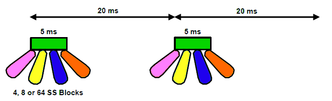
SS Block is transmitted over a limited bandwidth but with a much larger periodicity compared to LTE CRS. It can be used for power measurements to estimate path loss and channel quality but due to limited bandwidth and low duty cycle, SS Block is not very suitable for more detailed channel sounding aimed at tracking channel properties that vary rapidly in time/frequency.

What are the advantages of using CSI-RS?

  • CSI-RSs consume fewer air interface resources to perform channel measurement/feedback.
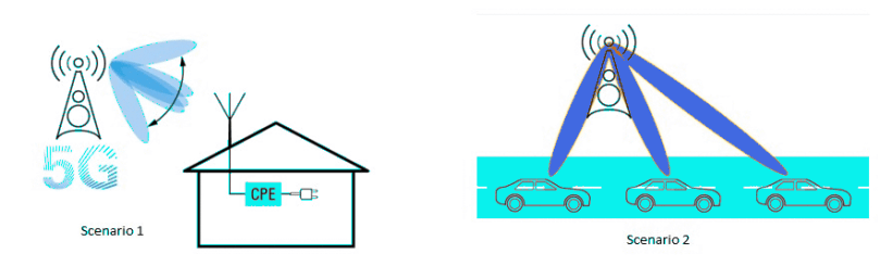
  • Different sets of CSI-RSs can be allocated to different UEs to form directional beams.

5G Base Stations can configure the UEs to use CSI-RS for:

  • Beam Management (CQI, RI, PMI Measurements): Measurements should be sent by UE to Base Stations in order to understand and estimate the correct direction of beams.
  • Connected Mode mobility: For calculating RSRP, RSRQ, SINR
  • Radio link failure detection: To check if channel is out of sync or in sync
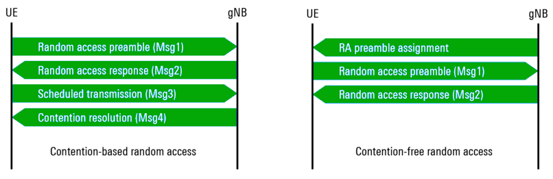
  • Beam failure detection and Recovery: Based on estimation of such signals, UE can be forced to perform contention free random-access attempt (when Base Station assigns dedicated preamble)
  • Time and Frequency Synchronization (Tracking Reference Signals)
  • Coordination and Multi Point transmission

CSI-RS Structure

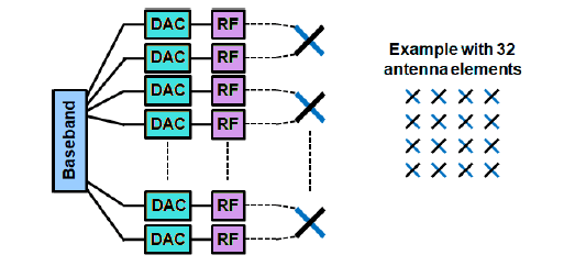
A configured CSI-RS may correspond to up to 32 antenna ports, each corresponding to a channel to be sounded. Depending on the number of antenna ports, there can be 2 possible arrangements:

  1. Single-Port: A single port CSI-RS occupies a single Resource element (RE) within a block corresponding to one slot in time domain and one resource block in frequency domain
  2. Multi-Port: multiple orthogonally transmitted per-antenna-port CSI-RS, sharing the overall set of REs assigned for the configured multi-port CSI-RS. Sharing can be based on combinations of: Code domain sharing CDM (different orthogonal patterns), Frequency Domain Sharing FDM (Different subcarriers within an OFDM symbol) or Time Domain Sharing TDM (Different OFDM symbols within a slot)

Below is an example showing single-port and multi-port CSIRS:

Single Port and Two port CSI-RS structure

Here, in case of Two-port CSI-RS Structure, we can see that how 2 adjacent RE’s in the frequency domain can be shared by means of CDM, which allows for code domain sharing between 2 per-antenna port CSIRS.

Below are the orthogonal patterns of each port:

 W0W1
1st Port+1+1
2nd Port+1-1

Note: CSI-RS can be configured to occur within an RB/slot block but to avoid collision with other downlink physical channels and signals with the same block, there are some restrictions. So, a UE/ Device can assume that the transmission of a configured CSI-RS will not collide with:

  • Any CORESET configured for the device,
  • Transmitted SS Blocks,
  • DMRS associated with the PDSCH transmissions scheduled for the device.

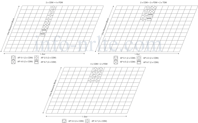
Taking example of 3 different structures for 8-port CSI-RS:

  • Frequency Domain CDM over 2 RE’s (2 x CDM) in combination with 4 times frequency multiplexing.
  • Frequency Domain CDM over 2 RE’s (2 x CDM) in combination with frequency and time multiplexing, consisting of 4 subcarriers with 2 OFDM symbols
  • Time and Frequency Domain CDM with 4 RE’s (4 x CDM) in combination with 2 times frequency multiplexing
8-Port CSI-RS
8-Port CSI-RS

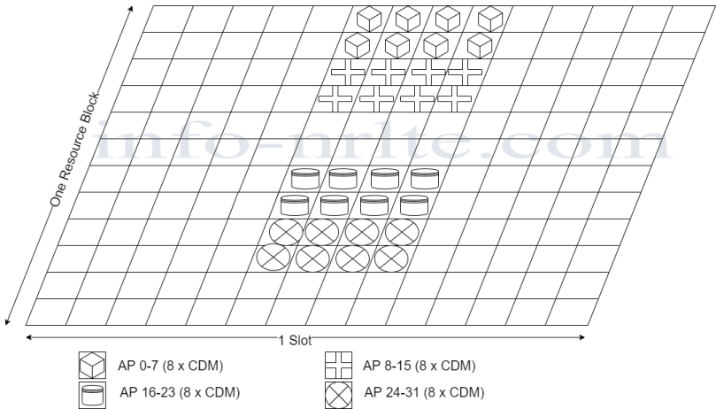
In the last example, we will consider one of possible structures of 32 port CSI-RS based on a combination of 8 x CDM and 4 times frequency multiplexing, which also suggests that CSI-RS antennas ports in the frequency domain need not occupy consecutive subcarriers. Similarly, CSI-RS ports separated in time domain need not occupy consecutive OFDM symbols.

32-Port CSI-RS
32-Port CSI-RS

CSI-RS Characteristics

CSI-RS are used for beamforming support, but they can be configured by layer 3 to be either beam-specific or UE specific. They are always mapped onto certain resources in frequency and time domain. These signals play an important role in performing tasks such as beam acquisition and evaluation, adaptation of the beam (beam refinement), decision making for beam switching and UE tracking with steerable beams.

The network could schedule the CSI-RS as a specific Reference Signals per beam to allow them to be distinguished from one another and on the other hand, RE’s carrying the CSI-RS can be configured to be either zero power (ZP-CSI-RS) or non-zero power (NZP-CSI-RS). One objective could be to provide a configuration that contains transmission gaps so that the UE can perform interference measurements and provide feedback. In addition, it may be used for optional beamforming implementations where the zero and non-zero power concept can be used to distinguish between beams.

NZP-CSI-RS is used for most of the procedures like Channel Measurement, Beam Management, Beam measurement, connected mode mobility etc. There is a dedicated signaling from BS to UE to configure the reception of such signals.

ZP-CSI-RS are special empty resource elements, used mostly for interference measurement. It defines a set of REs which do not contain any transmission for the UE. These REs may however contain transmissions for other UE so the name ‘Zero Power’ can be misleading. The important point is that these REs puncture the PDSCH so the UE does not expect to receive any DL data within them, i.e. ZP-CSI-RS are used to configure a RE puncturing pattern for the PDSCH when some REs are allocated for other purposes.

Below figure shows a possible usage example for such a mapping of ZP-CSI-RS and NZP-CSI-RS. Assuming a beam mobility condition, the gNB here used 2 beams with identical physical layer settings such as the bandwidth part and CORESET definition as well as the CSI-RS resources. gNB has configured the CSI-RS resources in an alternating mapping such that for each CSI-RS Instance in the time domain, only one of the 2 beams would have a non-zero CSI-RS.

Example of ZP-CSI-RS and NZP-CSI-RS

Here, UE must decide which beam is the best, means having the highest CSI-RSRP per beam. So, based on the CQI reports in the uplink direction, gNB can decide which beam to use and whether to apply a beam switching procedure.

CSI-RS Resource Sets

In addition to being configured with CSI-RS, a device can be configured with one or several CSI-RS resource sets, officially referred to as NZP-CSI-RS-ResourceSets. Each such resource set includes references to one or several configured CSI-RS. The resource set can then be used as part of report configurations describing measurements and corresponding reporting to be done by a device. Also, NZP-CSI-RS-ResourceSet may include pointers to a set of SS blocks, which suggests that some device measurements, especially measurements related to beam management and mobility, may be carried out on either CSI-RS or SS block.

CSI-RS Resource Indicator

The UE can be configured with a set of NZP-CSI-RS resources out of which it may be asked to report a subset. The identification of such NZP-CSI-RS is done by a CSI-RS RI. When a UE is configured with more than one nonzero-power CSI-RSs, it can report a set of N UE-selected CSI-RS resource-related indices. CRI can be used during Beam Management procedures when identifying the best downlink beam(s). The

CRI allow the Base Station to switch between CSI Reference Signal beams which are typically more directional than SS/PBCH beams. This is a very useful indicator as it can quickly point to the N best CSI-RS resources the network can use further.

CSI Related Measurements

CSI-RSRP

CSI Reference Signal Received Power measurements are used for connected mode mobility, power control calculations, and beam management. Measurements can be generated and reported at both layer I and layer 3. For example, a UE can provide CSI-RSRP measurements at Layer I when sending CSI to the BS. Alternatively, a UE can provide CSI-RSRP measurements at Layer 3 when sending an RRC Measurement Report. CSI-RSRP represents the average power received from a single RE allocated to the CSI-RS. Measurements are filtered at Layer 1 to help remove the impact of noise and to improve measurement accuracy.

CSI-RSRQ

CSI Reference Signal Received Quality measurements can be used for mobility procedures. In contrast to RSRP measurements, RSRQ measurements are not used when reporting CSI. CSI-RSRQ is defined as:

CSI-RSRQ = CSI-RSRP / (RSSI / N)

where N is the number of Resource Blocks across which the Received Signal Strength Indicator (RSSI) is measured, i.e. RSSI / N defines the RSSI per Resource Block. The RSSI represents the total received power from all sources including interference and noise. The RSRP and RSSl are both measured across the same set of Resource Blocks. The RSSI is measured during symbols which contain CSI RS REs.

CSI-SINR

CSl-RS Signal to interference and Noise Ratio measurements can be used for connected mode mobility

procedures. The CSI-SINR represents the ratio of the wanted signal power to the interference plus noise power. Both the wanted signal power and the interference plus noise power are measured from REs used by the CSI-RS.

Properties of Different CSI Configurations

Frequency Domain Property

A CSI-RS is configured for a given DL Bandwidth Part (BWP) and is then assumed to be confined within that BWP and use the numerology associated with that BWP. It can be configured to cover the full BW of the BWP or just a fraction of the BW. In the latter case, the CSI-RS bandwidth and frequency-domain starting position are provided as part of the CSI-RS configuration. Within the configured CSI-RS bandwidth, a CSI-RS may be configured for transmission in every resource block, referred to as CSI-RS density equal to one.

However, a CSI-RS may also be configured for transmission only in every alternate resource block, referred to as CSI-RS density equal to 1/2. In the latter case, the CSI-RS configuration includes information about the set of resource blocks (odd resource blocks or even resource blocks) within which the CSI-RS will be transmitted. CSI-RS density equal to 1/2 is not supported for CSI-RS with 4, 8, and 12 antenna ports.

There is also a possibility to configure a single-port CSI-RS with a density of 3 in which case the CSI-RS occupies three subcarriers within each resource block. This CSI-RS structure is used as part of a so-called Tracking Reference signal (TRS)

Time Domain Property

The per-resource-block CSI-RS structure mentioned above describes the structure of a CSI-RS transmission, assuming the CSI-RS is transmitted in a particular slot. In general, a CSI-RS can be configured for aperiodic, periodic, or semi-persistent transmission.

In the case of aperiodic CSI-RS transmission, no periodicity is configured. Rather, a device is explicitly informed (“triggered”) about each CSI-RS transmission instant by means of signaling in the DCI.

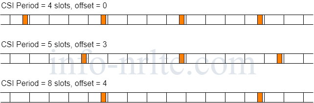
In the case of periodic CSI-RS transmission, a device can assume that a configured CSI-RS transmission occurs every Nth slot, where N ranges from as low as 4, that is, CSI-RS transmissions every 4th slot, to as high as 640, that is, CSI-RS transmission only every 640th  slot. In addition to the periodicity, the device is also configured with a specific slot offset for the CSI-RS transmission. It is based on RRC measurement.

Example of CSI-RS Transmission
Example of Periodic CSI-RS Transmission

In the case of semi-persistent CSI-RS transmission, a certain CSI-RS periodicity and corresponding slot offset are configured in the same way as for periodic CSI-RS transmission. However, actual CSI-RS transmission can be activated/ deactivated based on MAC control elements (MAC CE). Once the CSI-RS transmission has been activated, the device can assume that the CSI-RS transmission will continue according to the configured periodicity until it is explicitly deactivated. Similarly, once the CSI-RS transmission has been deactivated, the device can assume that there will be no CSI-RS transmissions according to the configuration until it is explicitly re-activated. It is also based on DCI signaling.

This periodic, semi-persistent or aperiodic transmission is not a property of the CSI-RS itself but rather the property of a CSI-RS resource set. So, activation/deactivation and triggering of semi-persistent and aperiodic CSI-RS, respectively, is not done for a specific CSI-RS but for the set of CSI-RS within a resource set.

Note: All CSI-RS within a semi-persistent resource set are jointly activated/ deactivated by means of a MAC CE command. Likewise, transmission of all CSI-RS within an aperiodic resource set is jointly triggered by means of DCI.

This article was just an introduction. I will come up later with an article related to CSI Measurement and reporting in detail.

References:

Dynamic TDD

Introduction to Duplexing Schemes in 5G NR

Duplex scheme implies the separation of transmission and reception or in other words, Uplink and Downlink data transmission. It is important that any cellular communications system must be able to transmit in both directions simultaneously. This enables conversations to be made, with either end being able to talk and listen as required. In order to be able to transmit in both directions, a device (UE) or base station must have a duplex scheme. To provide highest possible flexibility, 5G NR supports various duplexing schemes such as Frequency Division Duplex (FDD), Time Division Duplex (TDD), Semi-static TDD and Dynamic TDD.

Below is the basic description of above-mentioned duplexing schemes:

  • Frequency Division Duplex (FDD): It means that a carrier is designated as paired spectrum having an Uplink and Downlink carrier. Data transfer is possible in both the directions simultaneously at the same time because of different carrier frequencies for different directions. Also, allocation of resources can be managed dynamically and assigned independently in either the UL or the DL direction. Paired Bands are used for FDD.

There is full set of slots in both UL and DL during each frame and transmissions can occur simultaneously within a cell. Duplex filters (transmission/reception filters) are used to isolate between UL and DL transmissions. There are 2 possibilities even with this duplex mode:

  1. Half Duplex Mode: For a certain frequency band, it is not possible to have simultaneous transmission and reception in both UL and DL within a cell. It allows for a simplified device implementation due to relaxed or no-duplex filters.
  2. Full Duplex Mode: For a certain frequency band, it is possible to have simultaneous transmission and reception in both UL and DL within a cell.

Note: This full/half capability is a property of the device and not the Base station as it can anyways operate in full duplex mode irrespective of the device capability.

One of the drawbacks of this scheme is that the band definition requires a guard band between UL and DL, and the receiver must be equipped with a duplex filter to suppress interference from the transmitter.

  • Time Division Duplex (TDD): In TDD, only one carrier frequency is used. Transmission/Reception in UL and DL occurs on same frequency but at different time slots. Time slots can be allocated either to the UL or the DL. Unpaired bands are used for TDD, where UL and DL transmissions are non-overlapping in time, both for a device and cell’s perspective.

Receiver complexity is reduced in this case as the duplex filter is not needed. Also, the channel is reciprocal, thereby allowing improved implementation of channel estimation and link adaptation mechanisms such as precoding and AMC as well as directive antennas, which is a major advantage specifically for Beamforming methods.

Typically, a time interval such as frame structure or slot structure is divided into UL and DL time intervals. In 5G NR, one slot consists of 14 OFDMA symbols considering normal CP length and the slot configuration indicates the type of slot: UL or DL. In LTE, UL/DL changes were only possible at subframe level. So, switching between UL and DL at OFDMA symbol level in 5G NR allows much greater flexibility but causes challenges in implementation due to shorter time intervals and faster switching times. Also, in this case allocation of UL and DL is still static, within the cell.

One of the drawbacks of this scheme is related to the type of synchronization due to inter-cell interference and the need for a guard time between the transition from the RX to TX to compensate for propagation delay.

Basic Duplexing Schemes
  • Semi-Static TDD: It introduces more flexibility than the static TDD. In TD-LTE, 7 possible UL/DL configurations were defined on 1 frame corresponding to 10ms frame but here higher layer configuration parameters can be used in 5G NR to achieve cell-specific or even UE-specific UL/DL allocation parameterization. So, the slot configuration is flexible and can be changed from time to time while maintaining the focus on inter-cell interference aspects.
  • Dynamic TDD: It is the most flexible concept for UL/DL configuration. It is the possibility of dynamic assignment and reassignment of time domain resources between the UL and DL transmission directions. It is fully dynamic and could be a use case for small cells or even for standalone or isolated indoor cells with overlapping coverage to neighbor cells and therefore less influence due to inter-cell interference.

It enables rapid traffic variations specifically in dense deployments with a relatively small number of users per cell. Consider a situation where a user (almost alone) in a cell wants to download a major object, so for that most of the resources should be utilized in the DL direction and only a small fraction in the UL direction. A major difference with LTE is that in LTE, UL and DL allocations doesn’t change over time.

Time Division Duplex in 5G NR

TDD operation will be the main duplex arrangement for higher frequencies in 5G. Lower frequencies will still be using FDD as the interference problems with large cells is reduced by having different frequencies in UL and DL.

Frequency Bands in NR

If UL and DL data transmission takes places at the same time, then there could be interference problems between devices or between base stations.

Interference problems with TDD

In case of Base station to Base station, a weak signal from the UE sending a UL signal is disturbed by another base station sending a strong signal while in case of Device to Device communication, two UEs close to each other disturb each other. One UE receives a weak signal from the base station at the same time as a UE transmits a strong signal to its base station. The interference is worse in larger cells as the power is high from both base stations and UEs. This is the reason that TDD is easier to use in smaller cells having lower power. Small indoor cells are also rather isolated from each other which makes them quite suitable for TDD operation.

The advantage with TDD in high frequency bands is that the UL/DL capacity can be adapted to the traffic pattern in the cell. By allocating more or less time for DL, the cell capacity can be adapted to the needs of the cell. In FDD, this is not possible as the frequency allocation in UL/DL is static. With the flexible TDD system in 5G NR, each cell can be configured independently of others to adapt to traffic patterns in the cell.

An essential aspect of any half-duplex system in general, is the possibility to provide a sufficiently large guard period (GP) or guard time, where neither DL nor UL transmissions occur. TDD is also a type of Half Duplex system. Guard Period is necessary for switching from DL to UL transmission and vice versa and is obtained by using slot formats where the DL ends sufficiently early prior to the start of the UL. The GP should also ensure that UL and DL transmissions do not interfere at the base station. This is handled by advancing the UL timing at the devices such that, at the base station, the last uplink subframe before the UL-to-DL switch, ends before the start of the first DL subframe. The UL timing of each device can be controlled by the base station by using the timing advance mechanism. The GP must be large enough to allow the device to receive the DL transmission and switch from reception to transmission before it starts the (timing-advanced) UL transmission. As the timing advance is proportional to the distance to the base station, a larger GP is required when operating in large cells compared to small cells.

Creation of Guard Period for TDD Operation

Also, the selection of Guard Period need to take interference between base stations into consideration. In a multicell network, intercell interference from DL transmissions in neighboring cells must decay to a sufficiently low level before the base station can start to receive UL transmissions. Hence a larger GP may be required as the last part of DL transmissions from distant base stations, otherwise it might interfere with UL transmission.

Dynamic TDD (in detail)

Dynamic TDD is supported, where the UL and DL transmissions are dynamically scheduled to adapt to actual traffic mix and load but requires coordination to avoid interference between cells, so that there is no fixed UL/DL allocation. The basic approach to dynamic TDD is for the device to monitor for DL control signaling and follow the scheduling decisions. If the UE is instructed to transmit, it transmits in the UL direction otherwise it will attempt to receive any DL transmissions. The UL-DL allocation is thus completely under the control of the scheduler and any traffic variations can be dynamically tracked. Since a half-duplex device can’t transmit and receive simultaneously, there a need to split the resources between 2 directions. In NR, 3 different signaling mechanisms provide information to the device on whether the resources are used for UL or DL transmission:

  • Dynamic signaling for the scheduled device

The basic principle here is for the device to monitor for control signaling in the DL and transmit/receive according to the received scheduling grants/assignments. It is up to the scheduler to ensure that a half-duplex device is not requested to simultaneously receive and transmit. It is simple and provides a flexible framework.

  • Semi static signaling through RRC

Consider a situation where network already have some prior information related to a certain UL/DL allocation. For Example: if it is known to a device that a certain set of OFDM symbols is assigned to UL transmissions, there is no need for the device to monitor for DL control signaling in the part of the DL slots overlapping with these symbols. This can help reducing the device power consumption. NR therefore provides the possibility to optionally signal the UL_DL allocation through RRC signaling.

The RRC-signaled pattern is expressed as a concatenation of up to two sequences of DL-flexible-UL, together spanning a configurable period from 0.5ms up to 10ms. Furthermore, 2 patterns can be configured, one cell-specific provided as part of system information and one signaled in a device-specific manner. The resulting pattern is obtained by combining these two where the dedicated pattern can further restrict the flexible symbols signaled in the cell-specific pattern to be either DL or UL. Only if both the cell-specific pattern and the device-specific pattern indicate flexible should the symbols be for flexible use.

Example of Cell-Specific and Device-Specific UL-DL Pattern
  • Dynamic slot-format indication shared by a group of devices

The concept here is to dynamically signal the current UL_DL allocation to a group of devices, monitoring a special downlink control message known as the slot-format indicator (SFI). Here also, the slot format can indicate the number of OFDM symbols that are DL, flexible or UL, and the message is valid for one or more slots. The SFI message will be received by a configured group of one or more devices and can be viewed as a pointer into an RRC-configured table where each row in the table is constructed from a set of predefined DL/flexible/UL patterns, with one slot duration. Upon receiving the SFI, the value is used as an index into the SFI table to obtain the UL_DL pattern for one or more slots.

Example of SFI table configuration
Example of SFI table configuration  

Since a dynamically scheduled device will know whether the carrier is currently used for UL or DL transmission from its scheduling assignment/grant, the group common SFI signaling is primarily intended for nonscheduled devices. In particular, it offers the possibility for the network to overrule periodic transmissions of uplink sounding reference signals (SRS) or downlink measurements on channel-state information reference signals (CSI-RS), where both type of signals are used for assessing the channel quality.

Different TDD Configurations

5G NR supports 3 different TDD configurations:

  1. Static TDD Configuration on a common basis per cell
  2. Semi-static configuration on a UE with dedicated higher layer signaling
  3. Dynamic allocation based on possibility to indicate a TDD slot via DCI Scheduling

Let’s discuss each, one by one in detail below:

Static TDD Configuration

Higher Layer signaling uses, for example, system information block SIB1 or ServingCell-ConfigCommon to provide an IE TDD-UL-DL-ConfigCommon that contains configuration information on a cell-specific level. In this, the slots and symbols are defined over a period of time that are dedicated to either the UL or DL or can be declared ‘Flexible’, thereby enabling the overwriting with dynamic TDD configuration information.  The IE TDD-UL-DL-ConfigCommon contains the following parameters:

  1. referenceSubcarrierSpacing: Used for dynamic TDD configuration. SFI-RNTI scheduled by DCI will use the reference SubCarrierSpacing to calculate the duration of scheduled slots.
  2. dl-UL-TransmissionPeriodicity: This is the slot configuration period in milliseconds to which the TDD Configuration applies. This time results in even number of slots depending on the SCS. Some of the possible values are: 0.5ms, 0.625ms, 1ms, 1.25ms, 2ms, 2.5ms, 5ms and 10ms.
  3. nrofDownlinkSlots: This is the number of slots with only Downlink symbols. The dl-UL-TransmissionPeriodicity starts with this number of DL slots that only contains DL symbols. The maximum number depends on the SubCarrierSpacing and transmission periodicity.
  4. nrofDownlinkSymbols: This is the number of downlink symbols, which is followed by DL-only slots within the transmission periodicity. Maximum value can be 14 symbols.
  5. nrofUplinkSlots: This is the number of slots with only UL symbols. This number describes the last number of slots within the total number of slots given by transmission periodicity.
  6. nrofUplinkSymbols: This is the possible number of UL symbols that precede the number of UL slots at the end of transmission periodicity.
Static UL/DL TDD Configuration

Note: It is possible to configure a second TDD Config pattern TDD-UL-DL-ConfigCommon2 with the same parameters. The 2nd pattern is concatenated onto the 1st pattern. Using this configuration, 2 different TDD Patterns with different UL/DL configuration values can be aligned.

Semi-Static TDD Configuration

As we discussed above, the IE TDD-UL-DL-ConfigCommon configures certain number of UL and DL slots within a time period. So, the remaining slots from total number of slots per time period, which are neither UL nor DL, can be considered ‘Flexible’.

With the help of another IE TDD-UL-DL-ConfigDedicated, the network may configure these flexible slots in a UE-specific manner. It contains a set of slot configuration where each slot in the configuration set is assigned an index. The configuration of such a slot can be all DL or UL or mixed (or ‘explicit’). If it is all DL or UL, then all the 14 OFDM symbols within this slot are unidirectional. If the configuration is explicit, there is nrofDownlinkSymbols parameter to indicate the number of initial downlink symbols in this slot and nrofUplinkSymbols parameter to indicate the number of final symbols in this slot in the UL direction.

Semi-static UL/DL TDD Configuration

Note: Semi-static TDD configuration is a method that allows certain degree of flexibility in UL/DL TDD allocation, with the benefit that configuration can be UE Specific, thereby allowing a sort of traffic adaptation.

Dynamic TDD Configuration

This is valid for the flexible slot within the common configuration only. However, if the slot is not configured, it will be considered flexible anyways and a full dynamic TDD system will be possible. Due to inter-cell interference issues, such a fully dynamic TDD system is likely deployed or present only in isolated or very small cells. Using DCI format2_0 scheduling, a very dynamic TDD Configuration can be achieved on short notice. This DCI message is attached with a CRC, scrambled with SFI-RNTI and may be sent to a group of UEs to notify about the slot format for TDD operations. The length of DCI format is configurable by upper layers and this overall method is Dynamic TDD configuration.

Slot Configurations in 5G NR

NR defines a wide range of slot formats defining which parts of a slot are used for UL or DL. Each slot format represents a combination of OFDM symbols denoting DL, UL and flexible. Slot configurations can be pre-indicated and assigned to a UE via higher layer.

Slot configuration in 5G NR

Using DCI format2_0 scheduling, a very dynamic TDD configuration can be achieved on short notice. As per TS 38.213, Slot configurations for Normal Cyclic Prefix is mentioned below in the table. In this table, a particular slot format index specifies the type of symbol within that slot. The type can be downlink ‘D’, uplink ‘U’ or flexible ‘F’, where flexible can be UL or DL or Guard Period.

Configurations for different slot formats

References:

“5G NR – The next generation wireless access technology” – By Erik Dahlman, Stefan Parkvall, Johan Sköld

https://sharetechnote.com

https://pixabay.com/photos/antenna-telephony-television-radio-5357958/

Massive MIMO and Beamforming

What is MIMO

MIMO (Multiple Input Multiple Output) antenna technology is a way of increasing the capacity of a radio link using multiple transmit antennas and multiple receive antennas. Due to multipath propagation and decorrelated paths between the transmitter and receiver, multiple data streams can be sent over the same radio channel, thus increasing the peak data rate per user along with the capacity of the cellular network. MIMO has been part of LTE since the 1st release. LTE started with a 2×2 MIMO which means 2 transmit antennas at the base station (BS) side and 2 receive antennas at the UE side. LTE allow applications of up to 8 spatial layers in DL direction and up to 4 spatial layers in UL direction. Commercial LTE networks tend to use 2 or 4 spatial layers.

MIMO can be implemented in many ways:

  • Diversity: Multiple transmit and receive antennas are used to increase coverage (increased signal to interference plus noise ratio, SINR). Transmit diversity means to have multiple antennas at the sending side and receive diversity means to have multiple antennas at the receiver side to increase the captured radio energy.
  • Spatial Multiplexing: When multiple antennas are used by both sender and receiver, multiple streams can be sent with different information for increased user data bit rate. Transmission of data uses several layers with small phase shift between the layers, enabling a receiver to decode the layers separately.
  • Beamforming (BF): Multiple transmit antennas will direct the radio energy in a narrow sector to increase the SINR and thereby increasing the coverage (or increase the bitrate to the UE at a certain distance from the BS).

If different data streams are sent to the same receiver, it is referred to as Single User MIMO (SU-MIMO), while if the data streams are transmitted to different users, it is referred to as Multi-User MIMO (MU-MIMO)

Difference between SU-MIMO and MU-MIMO

With 5G NR, there is possibility of having up to 256 transmit antenna at the BS side and that is where the term ‘massive MIMO’ comes into picture. Massive MIMO antennas uses a large number of antenna elements but operate at frequencies below 6 GHz. Essentially, they exploit many elements to realize a combination of BF and spatial multiplexing.

Beamforming (BF) Fundamentals

Beamforming is a well-known and established antenna technology. Cellular networks such as LTE apply this technology to improve overall performance. Objects are identified by radar applications using Beamforming. It has more importance in 5G cellular communications as it allows deployment of 5G in higher frequency ranges such as cm-wave and mm-wave frequency spectrum where it is necessary to achieve enough cell coverage i.e. to compensate for high path loss at these frequencies.

The ability to steer beams dynamically is equally important since blockage scenarios are likely to occur due to moving objects such as cars or even a human body which can block the line of sight path. Consider some examples below:

  • In a fixed wireless access scenario, the customer premises equipment (CPE) in a household connects to an outdoor 5G BS. Here, no mobility is involved and a beam sweeping procedure would identify the best beam to be used.
  • In contrast, Beamforming needs to be dynamic (steerable or switchable) when a moving car on a road is connected.
Beamforming Scenarios

Support for BF is an essential capability in 5G NR which impacts the physical layer and higher layer resources. It is based on 2 fundamental physical resources: SS/PBCH blocks and the capability to configure channel state information reference signals (CSI-RS).

The principle of BF is to use the large number of antennas in, for example, an array. Each antenna can be controlled with a phase shifter and an attenuator. The antennas are usually half a wavelength of the signals they are optimized for. The phase of each antenna is then adjusted in order to control the direction of the beam. Preferably, the beam should be sent in the same direction as the UE transmitted in the UL. This means that the antennas and the logic controlling them must be able to measure the so called ‘angle of arrival’. If a signal comes from a direction in front of the antenna, all elements will receive a phase front of the signal at the same time. For Example: if the angle is 45 degrees, the antennas will receive the phase front of the signal with the time spread. By measuring the time delay between the arriving phase front to the antennas, it is possible to calculate the angle of arrival. To send the signal in the same direction, the phase front of the transmitted signal should be sent with the same time spread. Phase shifting can be done in the digital domain or analog domain.

Example of Phase array feeding network for BF with time dispersion of transmitted signal

Beamforming in 5G NR should be able to direct beams not only in horizontal direction but vertical direction as well, which is sometimes referred to as 3D MIMO as well. To be able to do that, antennas need to be put in a square, termed as Uniform Square Array (USA). Below is an example of 128 cross polarized antennas:

Uniform Square Array

By having the possibility to pack antennas and radio equipment very tightly, it is now possible to create antenna solutions with integrated antennas, analog to digital converters and power amplifiers. The antennas are put in a USA with cross-polarized antennas with 32, 64 or 256 antennas. Behind the Digital-to-analog-converter (DAC) is the baseband part which creates and analyzes the signals in the digital form, which comprises of number of Digital signal processors (DSP) with high capacity.

Example of Massive MIMO Based solution

As mentioned above, by measuring the phase front of the signal arriving to different antenna elements, it is possible to measure from which direction the signal comes in (Angle or arrival). To direct the radio energy in the same direction back to the UE, the same principle is used. This means that beams will be created from the antenna in different directions. By using different combinations of antennas, different beams can be created at the same time to different UEs located in different directions. However, the number of power amplifiers behind the antennas decide how many simultaneous beams can be created by the antenna. For Example: 8 beams can be created with 8 power amplifiers. The challenge is to pack amplifiers in an antenna and to reduce/remove the heat created by them as well as to limit the disturbance they cause to each other.

As a matrix is used, it is also possible to change the direction of the radio beam in both horizontal and vertical directions. In some case, it is referred to as 3D Beam Forming. This concept of creating beams from a Base Station will be a necessity in 5G NR when operating in very high frequency bands (FR2) due to bad radio propagation properties in these bands.

Similar principle can also be used on the receiver side in the UE or in the gNB receiver. The phase array can be set to amplify a signal arriving from a certain direction, which means that the receiver can focus on its antenna in a specific direction which is also referred to as Receiver side beam forming.

Operations in Beam Management

  • Beam Measurement: UE provides measurement reports to the Base Station on a per beam basis.
  • Beam Detection: UE identifies the best beam based on power measurements related to configured thresholds.
  • Beam Recovery: UE is configured with basic information to recover a beam in case the connection is lost.
  • Beam Sweeping: Using multiple beams at the Base Station to cover a geographic area and sweep through them at prespecified intervals.
  • Beam Switching: UE switches between different beams to support mobility scenarios.

Types of Beamforming

  • Analog BF: In this implementation, the baseband signal is 1st modulated then amplified and then split among the available number of antennas. Each RF chain has the capability to change the amplitude and phase individually. Analog BF in the RF path is simple and uses a minimal amount of hardware, making it the most cost-effective way to build a BF array. The drawback is that system can only handle one data stream and generate one signal beam. The beams must be time multiplexed and beams pointing in different directions are separated in time.
  • Digital BF: In this implementation, multiple digital streams are already generated in the baseband and as before, each is individually modified in phase and amplitude to generate the desired beam. So, several sets can be created and superimposed before feeding the array elements. This mechanism enables one antenna to generate multiple beams, each with its own signal and serving multiple users. Here, phase shifting is done before the Digital to Analog Conversion. BF modifications of the signals will be made in DSP by modifying the digital representation of the signal. This is the preferred method for lower frequencies in 5G as the advantage is that the phase and amplitude of each antenna can be controlled separately giving high flexibility. If each antenna can be controlled, full flexibility is possible with the number of beams the antenna can create at the same time. Here, phase shifting is done before the Digital to Analog Conversion. BF modifications of the signals will be made in DSP by modifying the digital representation of the signal. This is the preferred method for lower frequencies in 5G as the advantage is that the phase and amplitude of each antenna can be controlled separately giving high flexibility. If each antenna can be controlled, full flexibility is possible with the number of beams the antenna can create at the same time.
Difference between Analog and Digital Beamforming
  • Hybrid BF: This implementation combines both the above-mentioned methods. A limited number of digital streams feed multiple analog beamformers, whereas each is connected to a subset of total elements in the antenna array, which provides a compromise between implementation complexity, cost and flexibility.
Difference between Analog, Hybrid and Digital Beamforming

Note: Digital BF seems to be the most obvious way to implement Spatial Multiplexing as same signal can be sent from all the antennas to a particular user, with possible variation in phase/amplitude per antenna or possible variation in phase/amplitude per subcarrier. This is particularly important for cases where there is no direct line of sight between the Base station and the user.

Evolution of Massive MIMO

It is generally acknowledged that network densification is one of the main solutions to the exploding demand for capacity. Densification, when defined as the number of antennas per unit area, can be achieved through multi‐antenna systems such as massive MIMO.

Network densification proposes the deployment of a large number of antennas per cell site, to form what is known as a ‘massive MIMO’ (multi‐user MIMO with very large antenna arrays) network, once the number of antennas exceeds the number of active UEs per cell. This emerging technology uses multiple co‐located antennas (up to a few hundred) to simultaneously serve / spatially multiplex several users in the same time‐frequency resource. As the aperture of the array grows with many antennas, the resolution of the array also increases. This effectively concentrates the transmitted power towards intended receivers, thus the transmit power can be made arbitrarily small, resulting in significant reductions in intra‐ and inter‐cell interference. Distributing antennas has also been shown to result in highest capacity.

The antennas used for the macro cells are 2×4 MIMO and those used for the small cells are 128×4 MIMO (i.e. Massive MIMO). According to DoCoMo, “the aim of using Massive MIMO is to bar jamming through the beamforming technology”.

Approach for Massive MIMO

The approach here is to base all the beams on the uplink channel estimation. Here, UE sends a pilot signal which will be a known signal and Base station estimates what it receives, and, on that basis, it estimates the channel for the users. Thus, Base station can find some well-matched estimates to the channel and there is no need to make assumptions from beginning as to how channel looks like. Base station can just measure what it sees. It is also scalable with many antennas. This approach is different from the conventional approach where different angular beams are tried and user reports the best one, which is not a very nice solution as there is possibility of a user to be at the boundary and it can cause too much inter-user interference.

If the number of applied antenna elements is significantly increased at the Base station, for example if 64 cross-polarized antennas are used, the network node becomes a massive MIMO BS. Even with the increased number of antenna elements, the number of spatial layers is not increased. 5G NR supports 8 layers on the DL and 4 layers on the UL. However, large number of antenna elements allows the combinations of beamforming with spatial multiplexing. So, Massive MIMO antennas enabled focused transmission and reception of signal energy in the smaller regions of space, which brings huge improvements in user throughput, capacity and energy efficiency, especially when combined with simultaneous scheduling of multiple users.

In the established sub-6 GHz frequency spectrum, Base Station apply a large number of TX/RX antenna elements to serve multiple users with parallel data streams with moderate antenna gains. In contrast, the high path loss attenuation in the cm-wave and mm-wave bands requires high antenna gains. Consequently, both the Base Station and UE antenna implementations focus on high gain and dynamic Beamforming algorithms i.e. all available TX elements are used to create a single beam.

Distributed MIMO

NR is ready to support distributed MIMO however the support was not complete in release 15. Distributed MIMO implies that the device can receive multiple independent physical data shared channels (PDSCHs) per slot to enable simultaneous data transmission from multiple transmission points to the same user which means that some MIMO layers are transmitted from one site while other layers are transmitted from another site.

Advantages of Massive MIMO

  • With a greater number of antennas, beam width will be smaller (Narrower Beam due to involvement of fewer multipath components) leading to higher reliability and lower latency. This essentially means that the number of lost packets would be less and hence lesser retransmissions.
  • Resource allocations are made simple in Massive MIMO. All subcarriers are good at all times. So, no need to schedule based on fading. Each user gets the whole bandwidth whenever needed.
  • Massive MIMO can be very useful with:
    • Mobile Broadband applications
      • Very high spectral efficiency, multiplex many users
      • Great improvements at the cell edge
    • Ultra-Reliable Low Latency Communication (URLLC)
      • Lesser lost packets, so Fewer retransmissions
      • more predictable performance in the networks
    • Massive Machine-Type Communication (mMTC)
      • Can extend coverage, more cost-efficient deployment by putting up fewer Base Station in order to reach all the sensors.
      • Can help reduce transmit power for battery powered devices

Limitations of Massive MIMO

  • Works only with Time Division Duplex (TDD) mode where you change between UL and DL on the same frequency and for that reason, you can measure the channel in the UL and use it also for DL transmission.
  • The performance of massive MIMO is limited by the finite and correlated scattering given the space constraints. The degrees of freedom of the system, solely determined by the spatial resolution of the antenna array, can reach saturation point. Also, in frequency division duplex (FDD) systems, channel estimation and feedback for a large number of antennas presents a challenge. Unless the channel structure is available at the BS, the prohibitive downlink channel training and feedback in FDD systems sets an upper limit on the number of BS antennas.
  • With Massive MIMO, there is a challenge of manufacturing many low cost, low-precision components which also affects how to approach testing and verification of the performance of these antennas since over the air test methods must generally be applied.

Since this was just an introduction article, I might write another one in future to cover up more details about Massive MIMO.

References

Random Access

Introduction

Random Access (RACH) is the procedure where the User Equipment (UE) wants to create an initial connection with the network. This is one of the common procedures present in all the earlier versions of mobile systems including GSM, GPRS, UMTS and LTE, with some changes in messages exchanged between the UE and the Network. This procedure is done for many different reasons:

  • UE wants to connect for outgoing call/data/sms
  • UE responds to paging for incoming call/data/sms
  • Request of other system information (SIB2 – SIB9)
  • Handover to a new cell
  • Need uplink synchronization (UE being idle from sometime and has not transferred data)
  • Scheduling request when no UL resources are reserved for UE (no PUCCH)
  • Beam Recovery

Like in LTE, it consists of 4 signals transmitted between the UE and the base station (gNB), shown below:

Signaling for Random Access procedure

Summary of the procedure is: UE selects a “preamble” (a code sequence) and sends it at a random time on a UL channel called Physical Random Access Channel (PRACH). UE will start monitoring the DL channel to see if the base station (gNB) answers the request to connect to the network. If not, UE will make a new attempt with the increased power.

Random Access Response (RAR) sent by the network indicates which preamble it is related to, the Timing Advance (TA) it should use, a scheduling grant for sending Message 3 and a temporary Cell Radio Network Temporary Identifier (TC-RNTI). Message 3 and Message 4 will be used to resolve an eventual collision between 2 or more UEs attempting to access the network with the same preamble in the same physical PRACH resource, which is done by a unique identity (Either the RAN identity or the Core Network identity).

Once the random access (RA) procedure is completed, UE moves to connected state and UE-NW communication can continue using normal dedicated transmission.

Here in this blog, i will mostly focus on the RA Procedure during the standalone mode.

Characteristics of Preamble Transmission

In 5G NR, transmission timing of UL transmission is typically controlled by the network by means of regularly provided time adjustment commands (called closed-loop timing control). Prior to preamble transmission, there is no closed-loop timing control in operation so there will be an uncertainty in the preamble reception timing which for larger cells could be in order of 100µs or even more. So, in general, it is up to gNB scheduler to ensure that there are no other transmissions in the UL resources in which preamble transmission may take place. Below are some of the terms/characteristics associated with preamble transmission:

1.      Guard Time

The distance to the base station is unknown, when the UE starts a RA procedure. But in a system using OFDM with strict timing of symbols, it is important that symbols from users arrive at the receiver approximately the same time. If not, the UL orthogonality gets lost within the cell. To handle this, PRACH must have a guard time so that the UEs far away in the cell can still send a preamble without disturbing another UEs UL transmission. The larger the cell is, the larger guard time should be. Below fig. shows the concept:

Guard time for random access channel

The guard time in 5G is not specified so it is up to the scheduler in the gNB to fix this by not scheduling other UEs for UL transmission.

Typically, normal UL transmissions are based on explicit scheduling grant, thereby enabling contention-free access while on the other hand, the initial random access is inherently contention based, which means that multiple UEs may initiate preamble transmission simultaneously.  So, the preamble should be able to handle such kind of a situation and allow for correct preamble reception when such collisions occurs.

2.      PRACH Resources

Preamble transmission can take place within a configurable subset of RACH slots that repeats itself every RACH configuration period, within a cell. Also, the amount of resources for the PRACH is configurable. If the cell is large, many UL requests will be made due to large number of users whereas for an isolated indoor cell, the amount of resources could be limited. The resource for PRACH is set in both time and frequency. Timing part indicates how often it is occurring in UL and the frequency part indicates how wide the resources are. RACH periodicity can be set between 10 and 160ms and this value indicates how often this pattern with resources is repeated (RACH Slot). Within each RACH Slot, there can be number of RACH occasions which specifies how many different resources there are for each slot.

Below is an example of PRACH Configuration:

Example of PRACH Configuration

3.      Preambles

PRACH preamble is constructed by concatenating several short sequences, each sequence being of the same length as an OFDM symbol for other NR UL signals. These short sequences can be processed using the same FFT sizes as other UL signals thus avoiding the need of dedicated PRACH Hardware. This format also enables handling of large frequency offsets, fast time varying channels, phase noise and several receiver analog beamforming candidates within one PRACH preamble reception. Preamble format is also part of the cell random-access configuration i.e. each cell is limited to a single preamble format.

There are number of different preamble types available in the specification. The reason for having different alternatives is to provide flexibility regarding capacity, coverage and time delay (cell size). There are two main type of preambles:

  • Long preamble for frequency range 1 (FR1)
    • has 1.25 or 5KHz subcarrier spacing
    • based on a sequence length L = 839
    • 1.25KHz takes 6 resource blocks in frequency domain whereas 5Khz takes 24 resource blocks in frequency domain
    • Intended to be used for macro deployments (Large Cells)
    • Preamble formats for long preamble:
Long Preamble Formats
  • Short preamble for both FR1 and FR2
    • can have subcarrier spacings of 15, 30, 60 or 120KHz
      • 15 kHz or 30 kHz in the case of operation below 6 GHz (FR1)
      • 60 kHz or 120 kHz in the case of operation in the higher NR frequency bands (FR2).
    • based on a sequence length L = 139
    • takes 12 resource blocks regardless of subcarrier spacing
    • Intended for small cells and indoor deployments
    • Preamble formats for short preamble:
Short Preamble Formats

Note: The short preambles are, in general, shorter than the long preambles and often span only a few OFDM symbols. In most cases, it is possible to have multiple preamble transmissions multiplexed in time within a single RACH slot. In other words, for short preambles there may not only be multiple RACH occasions in the frequency domain but also in the time domain within a single RACH slot.

4.      PRACH and Beam forming

The possibility to establish a suitable beam pair during the initial access phase itself and to apply the receiver side analog beam sweeping for the preamble reception is a key feature of 5G NR initial access and is different from LTE.

During the initial access to a cell, it is beneficial if the base station (gNB) knows which beam the UE is receiving as the strongest. This is done by connecting a specific instance of SSB (synchronization signal block) to a specific beam. The measurements are done on SSB, when the UE measures on several detectable beams. Each SSB has a parameter ‘time index’ which makes it unique. By connecting an SSB time index with a specific RACH resource (slot and/or preamble), the UE will use that when accessing the cell. The base station (gNB) then knows which beam the UE prefers.

Beam establishment during initial access is enabled by the possibility of associating different SSB time indices with different RACH time/frequency occasions and/or different preamble sequences. As different SSB time indices in practice correspond to SSB transmissions in different DL beams, this means that the network, based on the received preamble, should be able to determine the DL beam in which the corresponding UE is located. This beam can then be used as an initial beam for subsequent DL transmissions to the UE.

Furthermore, if the association between SSB time index and RACH occasion is such that a given time-domain RACH occasion corresponds to one specific SSB time index, the network will know when, in time, preamble transmission from UEs within a specific DL beam will take place. Assuming beam correspondence, the network can then focus the UL receiver beam in the corresponding direction for beam-formed preamble reception. This implies that the receiver beam will be swept over the coverage area synchronized with the corresponding DL beam sweep for the SS-block transmission.

Note: Beam-sweeping for preamble transmission is only relevant when analog beamforming is applied at the receiver side. If digital beamforming is applied, beam-formed preamble reception can be done from multiple directions simultaneously.

5.      Preamble power control and Power Ramping

Generally, Preamble transmission takes place with a relatively large uncertainty in the required preamble transmit power. Therefore, Preamble transmission includes a power-ramping mechanism where the preamble may be repeatedly transmitted with a transmit power that is increased between each transmission. UE selects the initial preamble transmit power based on estimates of the DL path loss in combination with a target received preamble power configured by the NW. The path loss should be estimated based on the received power of the SSB that the UE has acquired and from which it has determined the RACH resource to use for the preamble transmission.

If no Random Access Response (RAR) is received within a predetermined window, the UE can assume that the preamble was not correctly received by the NW, and the reason might be that the preamble was transmitted with too low power. If this happens, the UE repeats the preamble transmission with the preamble transmit power increased by a certain configurable offset. This power ramping continues until a RAR has been received or until a configurable maximum number of retransmissions has been carried out, alternatively a configurable maximum preamble transmit power has been reached. In the two latter cases, the random-access attempt is declared as a failure.

Below fig. shows the setting for each preamble format. Depending on the counter of transmission of preamble, the power is increased further as the current counter setting is multiplied by the signaled power ramping step, which can have values as 0 dB, 2 dB, 4 dB or 6 dB. The maximum number of preamble transmissions is also signaled to the UE and is equal to 3, 4, 5, 6, 7, 8, 10, 20, 50, 100 or 200 transmissions.

Preamble Power Values for different preamble formats

Type of Random Access procedures in 5G NR

Like LTE, 5G NR uses a contention based random access (CBRA) or contention free random access (CFRA) procedure.

Contention Based and Contention Free random Access

CFRA is the mode which UE initially uses to perform the RA procedure in Non standalone mode. UE uses an assigned preamble to perform RA and the procedure finishes once the UE receives RAR. CBRA is the fallback scenario in NSA mode. If CFRA fails e.g. if the transmission of the dedicated preamble is not acknowledged, within a configured time period, then UE may switch to CBRA to establish UL synchronization. CFRA is typically applied when the UE is already in CONNECTED mode. Below table provides an overview of different use cases for each procedure:

Use Cases for Random Access Procedures

Fundamental difference between LTE and 5G NR regarding RA procedure is that the transmission of RA preamble for initial access is typically tied to the reception of the SSB in DL. In other words, UE preforms the signal quality measurements on the surrounding NR cells and decides the best received SSB (beam) index. The identified index determines on which frequency-time resource the RA preamble is transmitted using the PRACH. This enable gNB to focus its subsequent DL transmission of RAR in the same direction. For CFRA, the procedure ends with the reception of RAR. For CBRA, UE uses the information provided by the RAR to begin initial transmission on the PUSCH (message 3) using the same beam direction as for preamble transmission. Consequently, gNB sends the contention resolution using the same beam direction as for message 2.

Random Access procedure in Standalone Mode

In Non standalone mode, UE is signaled which RACH resource and preamble to use to perform Random Access procedure. For standalone mode, applying contention based random access (CBRA) the UE has to select a preamble and identify the frequency and time resources on the UL to transmit the preamble based on the results of signal quality measurements carried on the detected synchronization signal block (SSB).

Generation of random access preamble in based on the settings and values provided in RACH-Config-Common and RACH-ConfigGeneric, which also provides prach-ConfigurationIndex and thus the UE knows what preamble to use as well as in which subframe of a radio frame (SFN), it is allowed to transmit the preamble along with how many RACH occasions are applicable.

  • So, when to transmit the RA preamble? – The answer comes from a generic parameter mentioned above prach-ConfigurationIndex present in RACH-ConfigGeneric, which informs UE not only about the preamble format to use but also the point in time in which to transmit the preamble in the UL. There are total of 256 indices (0 to 255) and the configuration of each index depends on the frequency range (FR1 or FR2) and for FR1, also the type of spectrum (paired or unpaired) utilized by the network. Refer to TS 38.211, section 6.3.3.2.

UE also uses the threshold (rsrp-ThresholdSSB) definition provided by RACH-Config­Common to identify the SSB it should consider for selecting the RA preamble.

As per TS 38.213, UE is provided with a number N of SSB blocks that are associated with 1 RACH occasion and a number R of contention-based preambles mapped to each SSB. These 2 numbers are provided to UE within RACH-ConfigCommon as ssb-perRACH-OccasionAndCB-PreamblesPerSSB. This is a 2-fold information element. First, it takes one of eight different values of N as N=1/8, ¼, ½, 1, 2, 4, 8 or 16. Consider a PRACH Configuration index as 133. This index defines 6 different RACH occasions. Let’s set N to 1/8, which means one SSB is associated with 8 consecutive RACH occasions. Furthermore, if msg1-FDM is set to 4, the 1st 2 RACH occasions are associated with the SSB with index #0. SSB Index #1 is associated with the following 2 RACH occasions (RO #2, RO #3).

RACH occasions in the frequency – time domain and their association with SSBs

RACH occasions in the frequency – time domain and their association with SSBs

Depending on the value of N, there can be different values of R (see TS 38.331). The 1st 4 possible values of N (1/8, ¼, ½, 1) allow 16 different values of R with a standard step size of 4, starting at n4, n8… etc. If N=2, R can assume one of the 8 different values with n4, n8…n32. If N is 4,8 or 16, the values of R are either in the range from 1 to 16, 1 to 8 or 1 to 4 respectively. For R=n8 means 8 preambles out of a total of 64 are associated with 1 SSB, starting with index 0. In other words, preambles 0 to 7 are associated with SSB index #0, preambles 8 to 15 are associated with SSB index #1 and so forth.

Random Access Response (RAR) Reception by UE

Network will acknowledge the reception of RA preamble by transmitting MSG2, which is Random Access Response (RAR) on the DL to the UE. RAR is transmitted as a conventional DL PDCCH/PDSCH transmission with the corresponding PDCCH transmitted within the common search space. The information on the configuration of the control channel PDCCH is provided as part of ServingCellConfigCommonSIB in SIB1 and thus the UE knows which frequency and time resources to monitor for PDCCH carrying a DCI format 1-0 for which CRC is scrambled with RA-RNTI. DCI provides the frequency and time resource information on which RAR is carried by Resource block.

Assuming the NW is able to accommodate the UE based on its previously sent preamble, it would send a Random Access Preamble Id (RAPID) along with associated RAR. The UE compares received RAPID with the sequence it had selected as the preamble. If both matches, the reception of RAR is considered successful. Following the RAPID is the RAR which provides the UE with several pieces of information mentioned below:

  • Information about the RA preamble sequence the network detected and for which the response is valid;
  • Timing correction calculated by the network based on the preamble receive timing;
  • Scheduling grant, indicating resources that UE will use for the transmission of the subsequent Message 3
  • A temporary identity, the TC-RNTI, used for further communication between UE and network. The identity is 16 bit long and can be in the range of 0001 to FFEF (hex).

If the network detects multiple RA attempts (from different UEs), the individual response messages can be combined in a single transmission. Therefore, the response message is scheduled on the DL-SCH and indicated on a PDCCH using an identity reserved for RAR, the RA-RNTI. The use of the RA-RNTI is also necessary as a UE may not have a unique identity in the form of an allocated C-RNTI.

If the UEs that performed RA in the same resource used different preambles, no collision will occur and from the DL signaling it is clear to which UE(s) the information is related. However, there is a certain probability of contention—that is, multiple UEs using the same RA preamble at the same time. In that case, multiple UEs will react upon the same DL response message leading to collision.

Upon reception of the RAR, the UE will adjust its UL transmission timing and continue to the third step. If CFRA using a dedicated preamble is used, then this is the last step of the RA procedure as there is no need to handle contention in this case. Moreover, the UE already has a unique identity allocated in the form of a C-RNTI.

In the case of DL beamforming, the RAR should follow the beamforming used for the SS block which was acquired during the initial cell search. This is important as the UE may use receive-side beamforming and it needs to know how to direct the receiver beam. By transmitting the RAR using the same beam as the SS block, the UE knows that it can use the same receiver beam as identified during the cell search.

Message 3 Transmission

After the 2nd step, the UE is time synchronized in the UL direction. However, before user data can be transmitted to/from the UE, a unique identity within the cell, the C-RNTI, must be assigned to the UE (unless the UE already has a C-RNTI assigned). Depending on the UE state, there may also be a need for additional message exchange for setting up the connection.

So, in the next step, the UE transmits the necessary messages to the gNB using the UL-SCH resources assigned in the RAR in the previous step. An important part of the UL message is the inclusion of a UE identity, as this identity is used as part of the contention-resolution mechanism in the 4th step. If the UE is already known by the radio-access network, that is, in RRC_CONNECTED or RRC_INACTIVE state, the already-assigned C-RNTI is used as the UE identity (The UE identity is included as a MAC control element on the UL-SCH). Otherwise, a core-network UE identifier is used and the gNB needs to involve the core network prior to responding to the UL message in step 4.

Contention Resolution with Connection Set Up (Message 4)

The last step in the RA procedure consists of a DL message for contention resolution. Note that, from the 2nd step, multiple UEs performing simultaneous RA attempts using the same preamble sequence in the 1st step, listen to the same response message in the 2nd step and therefore have the same temporary identifier. Hence, the 4th step in the RA procedure is a contention-resolution step to ensure that a UE does not incorrectly use another UE’s identity.

The contention resolution mechanism differs somewhat depending on whether the UE already has a valid identity in the form of a C-RNTI or not. Note that the network knows from the UL message received in step 3 whether the UE has a valid C-RNTI or not. If the UE already had a C-RNTI assigned, contention resolution is handled by addressing the UE on the PDCCH using the C-RNTI. Upon detection of its C-RNTI on the PDCCH, the UE will declare the RA attempt successful and there is no need for contention-resolution-related information on the DL-SCH. Since the C-RNTI is unique to one UE, unintended UEs will ignore this PDCCH transmission.

If the UE does not have a valid C-RNTI, the contention resolution message is addressed using the TC-RNTI and the associated DL-SCH contains the contention-resolution message. Upon reception of Message 3, the MAC layer at the UE starts the ra-ContentionResolutionTimer. The value of contention resolution timer is provided with RACH-ConfigCommon. After starting the timer, UE begins monitoring the PDCCH for DCI format 1_0 with the CRC scrambled with corresponding TC-RNTI. Upon reception of the PDSCH, timer is stopped. If the decoded MAC PDU contains a Contention Resolution Identity (48 bits) that matches the CCCH SDU transmitted in Message 3, the contention resolution is considered successful. Furthermore, the C-RNTI is set to the previously temporary identity (TC-RNTI) and RA procedure is considered to be executed successfully.  In response to PDSCH reception, UE transmits an HARQ-ACK on the PUCCH. The PUCCH transmission is on the same initial bandwidth part as the Message 3 PUSCH transmission.

UEs that do not detect PDCCH transmission with their C-RNTI or do not find a match between the identity received in the 4th step and the respective identity transmitted as part of the 3rd step are considered to have failed the RA procedure and need to restart the procedure from the 1st step. No HARQ feedback is transmitted from these UEs. Moreover, a UE that has not received the DL message in step 4 within a certain time from the transmission of the UL message in step 3 will declare the RA procedure as failed and need to restart from the 1st step.

References:

Cell Search

Introduction

When a User Equipment(UE) is powered on or when it enters a new cell, it must be able to find the cell and synchronize to it in frequency and time. It must also be able to read some system information describing the cell in order to see if it can be used by the UE.

5G NR uses below synchronization signals:

  • Primary Synchronization Signal, PSS, with 3 different code sequences
  • Secondary Synchronization Signal, SSS, with 336 different code sequences

These signals enable the UE to find a cell along with helping it in synchronizing to the cell’s timing. There can be 1008 (3 X 336) possible code sequences and the value in the PSS/SSS determines cell’s Physical Cell Identity (PCI). When the UE finds these synchronization signals, it can also read the Physical Broadcast Channel (PBCH), whose location can be found around these synchronization signals.

Cell search also covers the functions and procedures by which a device finds new cells. The procedure is carried out when a device is initially entering the coverage area of a system. To enable mobility, cell search procedure is also continuously carried out by devices moving within the system, both when the device is connected to the network and when in idle/inactive state.

Cell Search in Standalone Mode

In order to perform the initial cell access in the Standalone (SA) mode, a UE need to perform Contention Based Random Access procedure (CBRA) and therefore it needs to acquire the relevant system information, which is System Information Block1 (SIB1). Accessing this information requires acquisition of Master Information Block (MIB) and it’s decoding. This is only possible while detecting and identifying the synchronization signal block. However, no information is provided in the SA mode to find the frequencies where the SSBs are transmitted, unlike Non-Standalone (NSA) mode where the UE receives the exact frequency location of the SSB via dedicated RRC signaling over the established LTE connection.

Synchronization Signal Block

A synchronization signal block (SSB) consists of one OFDM symbol for the PSS and one OFDM symbol for the SSS. Furthermore, the SS block may contain two OFDM symbols for the PBCH which are identical. So, the SS block spans four OFDM symbols in the time domain and 240 subcarriers in the frequency domain. PSS is transmitted in the first OFDM symbol of the SS block and occupies 127 subcarriers in the frequency domain. The remaining subcarriers are empty. SSS is transmitted in the third OFDM symbol of the SS block and occupies the same set of subcarriers as the PSS. There are eight and nine empty subcarriers on each side of the SSS. PBCH is transmitted within the second and fourth OFDM symbols of the SS block. In addition, PBCH transmission also uses 48 subcarriers on each side of the SSS. The total number of resource elements used for PBCH transmission per SS block thus equals 576, which includes resource elements for the PBCH along with resource elements for the demodulation reference signals (DMRS) needed for coherent demodulation of the PBCH.

Structure of SS Block

The synchronization signals and the physical broadcast channel within a synchronization signal block are time multiplexed. Below fig. shows another way of representing structure of SSB.

Synchronization signal block

One important difference between the SS block and the corresponding signals for LTE is the possibility to apply beam-sweeping for SS-block transmission i.e. the possibility to transmit SS blocks in different beams in a time-multiplexed fashion.

The timing of the SS Block can be set by the network operator. Default value of SSB transmission is 20ms but can be set between 5 and 160ms (5, 10, 20, 40, 80 and 160). During this time set by the operator, a number of SS Blocks will be transmitted in different directions (called Beams) during a 5ms Period. Each block of transmitted SS Blocks is referred to as an SS Burst Set. Although the periodicity of the SS burst set is flexible with a minimum period of 5ms and a maximum period of 160ms, each SS burst set is always confined to a 5ms time interval, either in the first or second half of a 10ms frame. Below example shows the default setting of 20ms.

Example of SS Block Timing with default setting

By applying beamforming for the SS block, the coverage of a single SS block transmission gets increased. Beam-sweeping for SS-block transmission also enables receiver-side beam-sweeping for the reception of uplink random-access transmissions as well as downlink beamforming for the random-access response

Now, the 20ms SS-block periodicity is four times longer than the corresponding 5ms periodicity of LTE PSS/SSS transmission. The longer SS-block period was selected to allow for enhanced NR network energy performance and in general to follow the ultra-lean design paradigm. The drawback with a longer SS-block period is that a device must stay on each frequency for a longer time in order to conclude that there is no PSS/SSS on the frequency. However, this is compensated for by the sparse synchronization raster which reduces the number of frequency-domain locations on which a device must search for an SS block.

SS Blocks can be sent over 4, 8 or 64 beams in a cell. The lower numbers will be used for lower frequencies as there will be a smaller number of antennas for such configuration. The SS Blocks will be used as follows:

  • 4 SS Blocks: used for frequency range 1 below 3 GHz
  • 8 SS Blocks: used for frequency range 1 between 3 and 6 GHz
  • 64 SS Blocks: used for frequency range 2

As per specifications, there can be different cases for the SS Block transmission. These cases cover different sub carrier spacings along with normal or extended cyclic prefix if the subcarrier spacing used is 30KHz. These cases are depicted below in the fig:

Different cases of SS Block Transmission

As you would have noticed, 60KHz subcarrier spacing is not included in above cases since it can’t carry any SS Blocks. Also, note that an SS Block is always distributed over 20 resource blocks in frequency domain. The size of the SS Block in the frequency domain will scale as per the subcarrier spacing used. Not all slots can be used for transmission of the block during the 5ms period when SS block can be transmitted. The number of slots used will also depend on the number of transmissions (4, 8 or 64) during the 5ms period. Below fig shows the possible transmission of SS Blocks for the case of 4 and 8 transmission times per 5ms period (depicted by the ‘L’ parameter in below fig)

Different options of SS Block Configuration

Difference between LTE and NR Cell Search Approach

In LTE, synchronization signals were located in the center of transmission BW so once an LTE device has found a PSS/SSS i.e. found a carrier, it inherently knows the center frequency of the found carrier. The drawback was that a device with no prior knowledge of the frequency-domain carrier position must search for PSS/SSS at all possible carrier positions (the “carrier raster”). So, a different approach has been adopted in 5G, to allow for faster cell search. In 5G, the signals are not fixed, rather located in a synchronization raster (a more limited set of possible locations of SS block within each frequency band). Instead of searching for an SS block at each position of the carrier raster, a device only needs to search for an SS block on the sparse synchronization raster. When found, the UE gets informed on where in frequency domain it is located.

Also, LTE used a concept of 2 synchronization signals with a fixed format which enabled UEs to find a cell. 5G NR also uses 2 synchronization signals but the difference is the support of beamforming and reduction in the number of “Always on” signals.

PSS and SSS

PSS is the first signal that a device entering the system will search for. At that stage, the device has no knowledge of the system timing. Once the device has found the PSS, it has found synchronization up to the periodicity of the PSS. PSS extends over 127 resource elements and has 3 different PSS Sequences. Physical cell identity (PCI) of the cell determines which of the three PSS sequences to use in a certain cell. When searching for new cells, a device must search for all three PSSs.

Once a device detects a PSS it knows the transmission timing of the SSS. By detecting the SSS, the device can determine the PCI of the detected cell. There are 1008 (3 X 336) different PCIs. However, already from the PSS detection the device has reduced the set of candidate PCIs by a factor 3. There are thus 336 different SSSs, that together with the already-detected PSS provides the full PCI. The basic structure of the SSS is same as that of the PSS i.e. the SSS consists of 127 subcarriers to which an SSS sequence is applied.

PBCH

While the PSS and SSS are physical signals with specific structures, PBCH is a more conventional physical channel on which explicit channel-coded information is transmitted. PBCH carries the MIB, which contains information that the device needs in order to be able to acquire the remaining SI broadcast by the network.

Below table shows the information carried by the PBCH:

Different options of SS Block Configuration
PBCH Contents
  • SS-block time index identifies the SS-block location within an SS burst set. Each SS block has a well-defined position within an SS burst set which is contained within the first or second half of a 5ms frame. From the SS-block time index, in combination with the half-frame bit, the device can determine the frame boundary. The SS-block time index is provided to the device as two parts:
    • 1st part encoded in the scrambling applied to the PBCH
    • 2nd part included in the PBCH payload.

For operation in higher NR frequency range (FR2), there can be up to 64 SS blocks within an SS burst set, implying the need for 3 additional bits to indicate the SS-block time index. These 3 bits are only needed for operation above 10 GHz and are included as explicit information within the PBCH payload.

  • CellBarred flag consist of two bits where 1st bit is the actual CellBarred flag that indicates whether devices can access the cell or not. Assuming devices are not allowed to access the cell, the 2nd bit, also referred to as the Intra-frequency-reselection flag, indicates whether access is permitted to other cells on the same frequency or not.
  • 1st PDSCH DMRS position indicates the time-domain position of the first DMRS symbol assuming DMRS Mapping Type A
  • SIB1 numerology provides info about the subcarrier spacing used for the transmission of the SIB1. The same numerology is also used for the downlink Message 2 and Message 4 that are part of the random-access procedure.
  • SIB1 configuration provides info about the search space, corresponding CORESET, and other PDCCH-related parameters that a device needs in order to monitor for the scheduling of SIB1.
  • CRB grid offset provides info about the frequency offset between the SS block and the common resource block grid. Information about the absolute position of the SS block within the overall carrier is provided within SIB1.
  • Half-frame bit indicates if the SS block is located in the 1st or 2nd 5ms part of a 10ms frame.

Acquiring System Information

When the UE has found the SS Block, it can read the PBCH which contains MIB. When the MIB has been decoded by the UE, it can start to search for SIB1. When SIB1 has been found and read, all remaining SIBs are decoded or requested.

In LTE, all system information was periodically broadcast over the entire cell area making it always available but also implying that it is transmitted even if there is no device within the cell. 5G NR, on the other hand, adopted a different approach where the system information, beyond the very limited information carried within the MIB, has been divided into two parts: SIB1 and the remaining SIBs.

SIB1 which is sometimes also referred to as the remaining minimum system information (RMSI) consists of the system information that a device needs to know before it can access the system. SIB1 is always periodically broadcast over the entire cell area. One important task of SIB1 is to provide the information the device needs in order to carry out an initial random access. SIB1 is provided by means of ordinary scheduled PDSCH transmissions with a periodicity of 160ms. The PBCH/MIB provides information about the numerology used for SIB1 transmission as well as the search space and corresponding CORESET used for scheduling of SIB1. Within that CORESET, the device then monitors for scheduling of SIB1 indicated by a special System Information RNTI (SI-RNTI).

In 5G a UE can request for other system information with a RACH procedure, as compared to the traditional mobile networks, where all other system information (SIB =>) is broadcasted. Below is the terminology that is used in 5G for the system information:

  • Minimum System Information
    • Master Information Block (MIB)
    • System Information Block1 (SIB1)
  • Other System Information
    • System Information Block 2 to 9 (SIB2 to SIB9)
Transmission of System Information

Minimum SI is always broadcasted in the whole cell. When Beamforming is used, the information is transmitted in all the beams. If a UE can’t decode the minimum SI, it should regard the cell as barred for access or camping.

Note: Small micro or Pico cells may not be used for initial access so the UEs must use a large macro cell for access and camping. The smaller cells may only be activated on demand when the traffic is high.

Other SI can be broadcasted but not always. This can be used in larger cells with high traffic.

As mentioned earlier, it is possible to request the other SI on-demand, which can be used in cells with low traffic. To request for the SI, the UE need to perform random access procedure. The network can either reserve dedicated resources for this request, or the UE will indicate the request for other system information in the message sent to the network. This way the network can avoid periodic broadcast of these SIBs in cells where no device is currently camping, thereby allowing for enhanced network energy performance.

Below is the short summary of the information carried by different SIBs:

  • SIB1: PLMN identity list, Tracking Area Code, Cell Identity, Barred/not Barred Indication, Cell Selection Information, SI scheduling information, support for emergency call indication, support for IMS voice call indication, timers, constants, barring information
  • SIB2: Cell reselection information
  • SIB3: Neighboring cells on same frequency (5G)
  • SIB4: Neighboring cells on different frequency (5G)
  • SIB5: Neighboring LTE cells
  • SIB6/7: ETWS information (Earthquake and Tsunami warning system)
  • SIB8: CMAS (Commercial Mobile Alert System)
  • SIB9: GPS and UTC Time

References:

  1. “5G NR – The next generation wireless access technology” – By Erik Dahlman, Stefan Parkvall, Johan Sköld
  2. http://www.techplayon.com/5g-nr-cell-search-and-synchronization-acquiring-system-information/
  3. http://howltestuffworks.blogspot.com/2019/10/5g-nr-synchronization-signalpbch-block.html

Carrier Aggregation

Introduction

Carrier Aggregation is a technology that aggregates multiple component carriers (CC), which can be jointly used for transmission to/from a single device. It combines two or more carriers into one data channel to enhance the data capacity of a network. Using existing spectrum, Carrier Aggregation helps mobile network operators (MNOs) in providing increased UL and DL data rates. When Carrier Aggregation is deployed, frame timing and SFN are aligned across cells that can be aggregated. 5G NR utilizes CA in both FR1 and FR2, supporting up to 16 component carriers. For Release 15, the maximum number of configured Component Carriers for a UE is 16 for DL and 16 for UL.

Important characteristics:

  • Up to 16 carriers (contiguous and non-contiguous) can be aggregated
  • Carriers can use different numerologies
  • Transport block mapping is per carrier
  • Cross carrier scheduling and joint feedback are also supported
  • Flexibility for network operators to deploy their licensed spectrum by using any of the CA types (such as intra-band contiguous, intra-band noncontiguous or inter-band noncontiguous)

History

LTE release 10 introduced enhanced LTE spectrum flexibility through carrier aggregation which was required to support higher bandwidths and fragmented spectra. Up to 5 component carriers, possibly each of different bandwidth, can be aggregated in this release, allowing for transmission bandwidths of up to 100MHz.  All component carriers need to have the same duplex scheme and in the case of TDD, same uplink downlink configuration.

In LTE release 10, Backwards compatibility was ensured as each component carrier uses the release-8 structure. Hence, to a release-8/9 device each component carrier will appear as an LTE release-8 carrier, while a carrier-aggregation capable device can exploit the total aggregated bandwidth, enabling higher data rates. In the general case, a different number of component carriers can be aggregated for the downlink and uplink. This was an important property from a device complexity point of view where aggregation can be supported in the downlink where very high data rates are needed without increasing the uplink complexity.

Release 13 marked the start of LTE Advanced Pro, included various enhancements in Carrier Aggregation. The number of component carriers possible to aggregate was increased to 32, resulting in a total bandwidth of 640MHz and a theoretical peak data rate around 25 Gbit/s in the DL considering 8 layers spatial multiplexing and 256 QAM. The main motivation for increasing the number of subcarriers was to allow for very large bandwidths in unlicensed spectra.

LTE release 13 also introduced license-assisted access, where the carrier aggregation framework is used to aggregate downlink carriers in unlicensed frequency bands, primarily in the 5 GHz range, with carriers in licensed frequency bands. Mobility, critical control signaling and services demanding high quality-of-service rely on carriers in the licensed spectra while (parts of) less demanding traffic can be handled by the carriers using unlicensed spectra.

In LTE release 14, license-assisted access was enhanced to address uplink transmissions also.

Carrier aggregation was one of the most successful enhancements of LTE till now with new combinations of frequency band added in every release.

Carrier Aggregation in NR

Like LTE, multiple NR carriers can be aggregated and transmitted in parallel to/from the same device, thereby allowing for an overall wider bandwidth and correspondingly higher per-link data rates. The carriers do not have to be contiguous in the frequency domain but can be dispersed, both in the same frequency band as well as in different frequency bands, resulting in three difference scenarios:

Intraband aggregation with frequency-contiguous component carriers;

Intraband aggregation with non-contiguous component carriers;

Interband aggregation with non-contiguous component carriers.

Below figure depicts these 3 scenarios:

Carrier Aggregation Types

Although the overall structure is the same for all three cases, the RF complexity can be vastly different.

Up to 16 carriers, having different bandwidths and different duplex schemes, can be aggregated allowing for overall transmission bandwidths of up to 6,400 MHz (16 x 400 MHz) = 6.4 GHz, which is more than typical spectrum allocations.

A device capable of CA may receive or transmit simultaneously on multiple component carriers while a device not capable of CA can access one of the component carriers. It is worth noting that in the case of Inter-band carrier aggregation of multiple half-duplex (TDD) carriers, the transmission direction on different carriers does not necessarily have to be the same. This implies that a carrier-aggregation-capable TDD device may need a duplex filter, unlike the typical scenario for a noncarrier-aggregation-capable device.

In the specifications, carrier aggregation is described using the term cell, that is, a carrier-aggregation-capable device can receive and transmit from/to multiple cells. One of these cells is referred to as the primary cell (PCell). This is the cell which the device initially finds and connects to, after which one or more secondary cells (SCells) can be configured, once the device is in connected mode. The secondary cells can be rapidly activated or deceived to meet the variations in the traffic pattern. Different devices may have different cells as their primary cell—that is, the configuration of the primary cell is device-specific. Furthermore, the number of carriers (or cells) does not have to be the same in UL and DL. In fact, a typical case is to have more carriers aggregated in the DL than in the UL. Reasons being:

  • There is typically more traffic in the DL that in the UL.
  • The RF complexity from multiple simultaneously active uplink carriers is typically larger than the corresponding complexity in the downlink.

Carrier aggregation uses L1/L2 control signaling for the same reason as when operating with a single carrier. As baseline, all the feedback is transmitted on the primary cell, motivated by the need to support asymmetric carrier aggregation with the number of downlink carriers supported by a device different than the number of uplink carriers. For many downlink component carriers, a single uplink carrier may carry a large number of acknowledgments. To avoid overloading a single carrier, it is possible to configure two PUCCH groups where feedback relating to the first group is transmitted in the uplink of the PCell and feedback relating to the other group of carriers is transmitted on the primary second cell (PSCell).

Multiple PUCCH Groups

If carrier aggregation is used, the device may receive and transmit on multiple carriers, but reception on multiple carriers is typically only needed for the highest data rates. It is therefore beneficial to inactivate reception of carriers not used while keeping the configuration intact. Activation and inactivation of component carriers can be done through MAC signaling containing a bitmap where each bit indicates whether a configured SCell should be activated or deactivated.

Difference between self-scheduling and cross-carrier scheduling

Scheduling grants and scheduling assignments can be transmitted on either the same cell as the corresponding data, known as self-scheduling, or on a different cell than the corresponding data, known as cross-carrier scheduling.

Self-scheduling vs Cross-scheduling

Let’s discuss in detail – the scheduling decisions are taken per carrier and the scheduling assignments are transmitted separately for each carrier, that is, a device scheduled to receive data from multiple carriers simultaneously receives multiple PDCCHs. A PDCCH received can either point to the same carrier, known as self-scheduling, or to another carrier, commonly referred to as cross-carrier scheduling or cross-scheduling. In case of cross-carrier scheduling of a carrier with a different numerology than the one upon which the PDCCH was transmitted, timing offsets in the scheduling assignment, for example, which slot the assignment relates to, are interpreted in the PDSCH numerology (and not the PDCCH numerology).

Carrier Aggregation support in MAC Layer

MAC Layer is responsible for multiplexing/demultiplexing data across multiple component carriers when carrier aggregation is used. In case of CA, it is responsible for distributing data from each flow across the different component carriers, or cells.

The basic principle for carrier aggregation is independent processing of the component carriers in the physical layer, including control signaling, scheduling and HARQ retransmissions, while carrier aggregation is invisible above the MAC layer. Carrier aggregation is therefore mainly seen in the MAC layer, where logical channels, including any MAC control elements, are multiplexed to form transport blocks per component carrier with each component carrier having its own HARQ entity.

Carrier Aggregation in MAC

Note: In the case of carrier aggregation, there is one DL-SCH (or UL-SCH) per component carrier seen by the device

Relation with Dual Connectivity

Dual connectivity implies that a device is simultaneously connected to two cells. User-plane aggregation, where the device is receiving data transmission from multiple sites, separation of control and user planes, and uplink-downlink separation where downlink transmissions originate from a different node than the uplink reception node are some examples of the benefits with dual connectivity. To some extent it can be seen as carrier aggregation extended to the case of non-ideal backhaul. It is also essential for NR when operating in non-standalone mode with LTE providing mobility and initial access.

Example of Dual Connectivity

In dual connectivity, a device is connected to two cells, or in general, two cell groups, the Master Cell Group (MCG) and the Secondary Cell Group (SCG). The reason for the term cell group is to cover also the case of carrier aggregation where there are multiple cells, one per aggregated carriers, in each cell group. The two cell groups can be handled by different gNBs.

Dual Connectivity Details

A radio bearer is typically handled by one of the cell groups, but there is also the possibility for split bearers, in which case one radio bearer is handled by both cell groups. In this case, PDCP is in charge of distributing the data between the MCG and the SCG and thus PDCP plays an important role for Dual connectivity support.

Differences between Dual Connectivity and Carrier Aggregation

Both carrier aggregation and dual connectivity result in the device being connected to more than one cell. Despite this similarity, there are fundamental differences, primarily related to how tightly the different cells are coordinated and whether they reside in the same or in different gNBs.

Carrier aggregation implies very tight coordination, with all the cells belonging to the same gNB. Scheduling decisions are taken jointly for all the cells the device is connected to by one joint scheduler. Dual connectivity, on the other hand, allows for a much looser coordination between the cells. The cells can belong to different gNBs, and they may even belong to different radio-access technologies as is the case for NR-LTE dual connectivity in case of non-standalone operation.

Carrier aggregation and dual connectivity can also be combined. This is the reason for the terms master cell group and secondary cell group. Within each of the cell groups, carrier aggregation can be used.

Multi Connectivity includes Dual Connectivity (PDCP UP Split) and Carrier Aggregation (MAC UP Split) as shown in the figure below:

Carrier Aggregation with Dual Connectivity

Dual Connectivity should be preferred when latency is not neglectable between paths i.e. > 5-10ms or when there is a different RAT to be connected and TN of the master side is congested, whereas Carrier Aggregation has better and faster utilization of radio resources than Dual Connectivity but is used to connect same RATs. It requires low inter site latency (<5ms).

Note:

  • In the case of carrier aggregation or dual connectivity, multiple power headroom reports can be contained in a single message (MAC control element).
  • NR does not support carrier aggregation with LTE and thus dual connectivity is needed to support aggregation of the LTE and NR throughput.
  • NR specifications supports carrier aggregation, where multiple carriers are present within a band, or in multiple bands, can be combined to create larger transmission bandwidths.

Relation with Supplementary Uplink

Both these techniques allow the uplink transmission to be switched between the FDD-band and the 3.5 GHz band. The use of these mechanisms effectively utilizes idle sub-3 GHz band resources, improve the uplink coverage of C-band, and enable the provisioning of 5G services in a wider area. Both solutions, NR Carrier Aggregation and Supplementary Uplink, offer transport of UL user data using sub-3GHz band NR radio resources. NR CA provides the added benefit of also providing sub-3GHz DL user data support on the FDD-band downlink, using 3GPP specified LTE-NR spectrum sharing, if needed. This provides opportunity to aggregate NR bandwidth as well as better operation of the NR uplink.

Difference between Carrier Aggregation (CA) and supplementary uplink (SUL)

Supplementary uplink differs from the aggregated uplink in that the UE may be scheduled to transmit either on the supplementary uplink or on the uplink of the carrier being supplemented, but not on both at the same time.

In a typical carrier aggregation scenario:

  • Main aim of carrier aggregation is to enable higher peak data rates by increasing the bandwidth available for transmission to/from a device.
  • The two (or more) carriers are often of similar bandwidth and operating at similar carrier frequencies, making aggregation of the throughput of the two carriers more beneficial. Each uplink carrier is operating with its own associated downlink carrier, simplifying the support for simultaneous scheduling of multiple uplink transmissions in parallel. Formally, each such downlink carrier corresponds to a cell of its own and thus different uplink carriers in a carrier-aggregation scenario correspond to different cells.

While in case of SUL scenario:

  • Main aim of SUL is to extend uplink coverage, that is, to provide higher uplink data rates in power-limited situations, by utilizing the lower path loss at lower frequencies
  • The supplementary uplink carrier does not have an associated downlink carrier of its own. Rather, the supplementary carrier and the conventional uplink carrier share the same downlink carrier.  Consequently, the supplementary uplink carrier does not correspond to a cell of its own. Instead, in the SUL scenario there is a single cell with one downlink carrier and two uplink carriers.
Carrier Aggregation vs Supplementary Uplink

Benefits of Carrier Aggregation

  • Better Network Performance: Carriers provide a more reliable and stronger service with less strain on individual networks.
  • Leveraging of underutilized spectrum: CA enables carriers to take advantage of underutilized and unlicensed spectrum, thereby extending the benefits of 5G NR to these bands.
  • Increased uplink and downlink data rates: Wider bandwidth mean higher data rates.
  • More efficient use of spectrum: Operators can combine fragmented smaller spectrum holdings into larger and more useful blocks and can create aggregated bandwidths greater than those that would be possible from a single component carrier.
  • Network carrier load balancing: Enables intelligent and dynamic load balancing with real‐time network load data.
  • Higher capacity: CA doubles the data rate for users while reducing latency with a good amount.
  • Scalability: Expanded coverage allows carriers to scale their networks rapidly.
  • Dynamic switching: CA enables dynamic flow switching across component carriers (CCs).
  • Better user experience: CA delivers a better user experience with higher peak data rates (particularly at cell edges), higher user data rates, and lower latency, as well as more capacity for “bursty” usage such as web browsing and streaming video.
  • Enabling of new mobile services: Delivering a better user experience opens opportunities for carriers to innovate and offer new high bandwidth/high data rate mobile services.
  • Can be combined with Dual Connectivity

Disadvantages/Challenges with Carrier Aggregation:

  • Intra‐band uplink CA signals use more bandwidth and have higher peak‐to‐average power ratios (PAPRs)
  • Many possible configurations of resource blocks (RBs) exist in multiple component carriers (CCs) where signals could mix and create spurious out‐of‐band problems.
  • Intra‐band CA signals present mobile device designers with many challenges because they can have higher peaks, more signal bandwidth, and new RB configurations. A Power Amplifier design must be tuned for very high linearity even though the signal power may be backed off. Adjacent channel leakage, intermodulation products of non‐contiguous RBs, spurious emissions, noise, and sensitivity must be considered. The tradeoff of linearity comes at the expense of efficiency and thermal effects.
  • Inter‐band CA combines transmit signals from different bands. The maximum total power transmitted from a mobile device is not increased in these cases, so for two transmit bands, each band carries half the power of a normal transmission, or 3 dB less than a non‐CA signal. Because different PAs are used to amplify the signals in different bands, and the transmit power is reduced for each, the PA linearity isn’t an issue. Other front‐end components, like switches, have to deal with high‐level signals from different bands that can mix and create intermodulation products. These new signals can interfere with one of the active cellular receivers or even another receiver on the phone, like the GPS receiver. To manage these signals, switches must have very high linearity.

References:

  1. https://www.gsma.com/futurenetworks/wp-content/uploads/2019/03/5G-Implementation-Guideline-v2.0-July-2019.pdf
  2. “5G NR – The next generation wireless access technology” – By Erik Dahlman, Stefan Parkvall, Johan Sköld
  3. https://www.3gpp.org/technologies/keywords-acronyms/101-carrier-aggregation-explained
  4. https://www.qorvo.com/design-hub/ebooks/5g-rf-for-dummies

HARQ

Introduction

5G NR (New radio) has several retransmission systems using three different layers in the protocol stack:

  • MAC protocol: It implements a fast retransmission system with delay less than 1ms in new radio, called HARQ (Hybrid Automatic Repeat reQuest).
  • RLC protocol: Even though HARQ is present at MAC but there might still be some possibility of errors in the feedback system. So, for dealing with those errors, RLC has a slow retransmission system but with a feedback protected by CRC. Compared to the HARQ acknowledgments, the RLC status reports are transmitted relatively infrequently.
  • PDCP protocol: This will guarantee in-sequence delivery of user data and it is mainly used during handover as RLC and MAC buffers are flushed when a handover is executed.

NR uses an asynchronous hybrid-ARQ protocol in both downlink and uplink, that is, the hybrid-ARQ process which the downlink or uplink transmission relates to is explicitly signaled as part of the downlink control information (DCI). The hybrid-ARQ mechanism in the MAC layer targets very fast retransmissions and, consequently, feedback on success or failure of the downlink transmission is provided to the gNB after each received transport block (for uplink transmission no explicit feedback needs to be transmitted as the receiver and scheduler are in the same node).

HARQ is implemented to correct the erroneous packets coming from PHY layer. If the received data is erroneous then the receiver buffers the data and requests for a re-transmission from the sender. When the receiver receives the re-transmitted data, it then combines it with buffered data prior to channel decoding and error detection. This helps in the performance of re-transmissions. For this to work, the sending entity need to buffer the transmitted data until the ACK is received since the data needs to be retransmitted in case a NACK is received.

HARQ is a stop and wait (SAW) protocol with multiple processes. The protocol will continue to repair one transmission without hindering other ongoing transmissions which can continue in parallel.

HARQ principle with multiple processes

Why multiple SAW processes are required?

Once a packet is sent from a process, it waits for an ACK/NACK. While it is waiting for an ACK/NACK in the active state, no other work can be done by the same process leading to reduced performance. So, if we have multiple such processes working in parallel, throughput can be increased by making other processes work at the same time on other packets, while a process is in waiting state for ACK/NACK.

Differences with LTE HARQ

  • New radio is using an asynchronous protocol in both UL and DL, which is different from LTE, where the protocol was synchronous in UL; UE should reply with an ACK/NACK after 3ms of receiving the DL data. The gNB knows that when the ACK/NACK is expected. In NR, the report timing is not fixed to increase the flexibility which is important for URLLC services.
  • PHICH (Physical HARQ Indicator channel) was used in LTE to handle uplink retransmissions and was tightly coupled to the use of a synchronous HARQ protocol, but since the NR HARQ protocol is asynchronous in both uplink and downlink the PHICH is not needed in NR.
  • In LTE, Non-adaptive retransmissions were triggered by a negative acknowledgement on the PHICH, which used the same set of resources as the previous transmission i.e. the modulation scheme and the set of allocated resource blocks remains unchanged. Only Redundancy version used to change between transmissions. But in NR, PHICH is not there and retransmissions are adaptive that can be triggered by DCI. NDI flag retriggers a transmission if its value is toggled relative to previous transmission.
  • Maximum number of HARQ processes was set to 8 in LTE but is increased to 16 in NR. This was motivated by shorter time slot and increased use of remote radio heads that will increase the round-trip time slightly.

Reasons why NR HARQ is asynchronous in both UL and DL:

  • Synchronous HARQ operation does not allow dynamic TDD.
  • Operation in unlicensed spectra (part of later NR releases) is more efficient with asynchronous operation as it is not guaranteed that the radio resources are available at the time for a synchronous transmission.

Hybrid ARQ with Soft combining

The hybrid-ARQ protocol is the primary way of handling retransmissions in NR. In case of an erroneously received packet, a retransmission is requested. However, despite it not being possible to decode the packet, the received signal still contains information, which is lost by discarding erroneously received packets. This shortcoming is addressed by hybrid-ARQ with soft combining. In hybrid- ARQ with soft combining, the erroneously received packet is stored in a buffer memory and later combined with the retransmission to obtain a single, combined packet that is more reliable than its constituents. Decoding of the error-correction code operates on the combined signal. Both Chase combining and Incremental Redundancy methods were proposed initially, but it is Incremental Redundancy that is getting used in NR.

Difference between Chase combining and Incremental Redundancy

In Chase combining, the physical layer applies the same puncturing pattern to both the original transmission and each retransmission. This results in retransmissions which include the same set of physical layer bits as the original transmission. Systematic bit remains the same even in the subsequent transmission. Only Parity 1 and Parity 2 bits are punctured. Benefits of chase combining are its simplicity and lower UE memory requirements.

Example of Chase Combining

In Incremental Redundancy, the physical layer applies different puncturing patterns to the original transmission and retransmission. This results in retransmission which include a different set of physical layer bits to the original transmission. 1st transmission provides the systematic bits with the greatest priority while subsequent retransmissions can provide either the systematic or the parity 1 and parity 2 bits with greatest priority. Drawbacks associated with Incremental Redundancy are its increased complexity and increased UE memory requirements.

Example of Incremental redundancy

Performance wise, incremental redundancy is like chase combining when the coding rate is low i.e. there is less puncturing. But, when there is an increased quantity of puncturing, the performance of incremental redundancy becomes greater i.e. when the coding rate is high because channel coding gain is greater than soft combining gain.

Codeblock Groups

Due to increased data rate in NR, when several gigabits per second is transmitted, the size of the transport block will be too large to handle. So, these transport blocks will be split into codeblocks, each with its own 24 bits CRC. This principle made it possible to handle large transport block in parallel channel coders/decoders.

In NR, there can be hundreds of codeblocks in a transport block. If only one or a few of them are in error, retransmitting the whole transport block results in a low spectral efficiency compared to retransmitting only the erroneous codeblocks.

To reduce the control signaling overhead, 2,4,6 or 8 blocks can be grouped together to Codeblock Groups (CBG). In case of an error in one Codeblock, only the Codeblock group to which the faulty Codeblock belongs, need to be retransmitted instead of whole transport block. If per-Code Block Group (per-CBG) retransmission is configured, feedback is provided per CBG instead of per transport block and only the erroneously received codeblock groups are retransmitted, which consumes less resources than retransmitting the whole transport block.

Retransmission of single Codeblock group

HARQ in Downlink

The gNB will send a scheduling message to the UE that indicates where the user data is located and how it is coded. Downlink Control Information (DCI) will indicate which HARQ process to be used by the UE. Since transmissions and retransmissions are scheduled using the same framework, the UE needs to know whether the transmission is a new transmission, in which case the soft buffer should be flushed, or a retransmission, in which case soft combining should be performed. For that purpose, a New Data Indicator (NDI) bit will also be set to indicate that this will be new data and the receive buffer should be flushed before loading the user data.

Upon reception of a downlink scheduling assignment, UE checks the new-data indicator to determine whether the current transmission should be soft combined with the received data currently in the soft buffer for the HARQ process in question, or if the soft buffer should be cleared. UE receives the user data and starts to calculate a checksum of the single transport block and if used, the included codeblocks. After completing the calculation, the UE follows the timing order of the UL report and sends an HARQ report indicating ACK or NACK. In case of NACK, the gNB will start to schedule a retransmission of the data.

HARQ in Downlink
Retransmission of code block in DL

Now if per- CBG retransmissions are configured, UE needs to know which CBGs are retransmitted and whether the corresponding soft buffer should be flushed or not. For this purpose, two additional fields are present in the DCI. 1) CBG Transmit Indicator (CBGTI), which is a bitmap indicating whether a certain CBG is present in the downlink transmission or not and 2) CBGFI which is a single bit, indicating whether the CBGs indicated by the CBGTI should be flushed or whether soft combining should be performed.

Example of per-CBG retransmission

The result of the decoding operation—a positive acknowledgment in the case of a successful decoding and a negative acknowledgment in the case of unsuccessful decoding—is fed back to the gNB as part of the uplink control information. If CBG retransmissions are configured, a bitmap with one bit per CBG is fed back instead of a single bit representing the whole transport block.

DCI Format 1-0 and 1-1 for downlink scheduling assignment contains HARQ related information as:

  • Hybrid-ARQ process number (4 bit), informing the device about the hybrid-ARQ process to use for soft combining.
  • Downlink assignment index (DAI, 0, 2, or 4 bit), only present in the case of a dynamic hybrid-ARQ codebook. DCI format 1_1 supports 0, 2, or 4 bits, while DCI format 1_0 uses 2 bits.
  • HARQ feedback timing (3 bit), providing information on when the hybrid- ARQ acknowledgment should be transmitted relative to the reception of the PDSCH.
  • CBG transmission indicator (CBGTI, 0, 2, 4, 6, or 8 bit), indicating the code block groups. Only present in DCI format 1_1 and only if CBG retransmissions are configured.
  • CBG flush information (CBGFI, 0_1 bit), indicating soft buffer flushing. Only present in DCI format 1_1 and only if CBG retransmissions are configured.

HARQ in Uplink

The gNB sends a scheduling message to the UE indicating resources to be used for uplink transmission, which also has HARQ process number. The UE will follow the order and send the transport block (or Codeblock group) as per the scheduling grant. The gNB will calculate and verify the checksum for the correctness of the message. The gNB will order the UE to retransmit the transport block again with a new scheduling grant, if an error id detected. In order to indicate a retransmission is required, same HARQ process number is sent with NDI bit set to no, which will be interpreted by the UE as retransmission.     

HARQ in UL
Retransmission of a transport block in UL

The CBGTI is used in a similar way as in the downlink to indicate the codeblock groups to retransmit in the case of per-CBG retransmission. Note that no CBGFI is needed in the uplink as the soft buffer is located in the gNB which can decide whether to flush the buffer or not, based on the scheduling decisions.

DCI format 0-0 and 0-1 for uplink scheduling grants also contains HARQ related information as:

  • Hybrid ARQ process number (4 bit), informing the device about the hybrid-ARQ process to (re)transmit.
  • Downlink assignment index (DAI), used for handling of hybrid-ARQ codebooks in case of UCI transmitted on PUSCH. Not present in DCI format 0_0.
  • CBG transmission indicator (CBGTI, 0, 2, 4, or 6 bit), indicating the code block groups to retransmit. Only present in DCI format 0_1 and only if CBG retransmissions are configured.

Timing of UL reports

The timing of the UL HARQ reports was fixed in LTE as 3ms, which was way too much for 5G and URLLC services. The solution in NR is to have a flexible solution that can be modified between different service requirements and when new HW is developed. The gNB informs the UE about the timing in a ‘HARQ timing’ field in the Downlink Control Information (DCI). This flexibility was also required in dynamic TDD when the directions of the slots is flexible (UL/DL). The “HARQ Timing” field contains a 3-bit pointer to an RRC Configured Table, which will indicate the timing between the scheduling message (The data this is included in the slot) and the related UL report. This will also allow for the gNB to order several transmissions to be grouped together or to order the UE to report as quickly as possible (for delay sensitive services). This information provides the UE with the information when to send the HARQ report back to the gNB.

Now where in the frequency band the information should be sent (Physical Uplink Control Channel, PUCCH)? The answer is that RRC protocol configures another table and the UE will get a pointer to the table in the scheduling message. This will tell the UE where to send the HARQ report.

Multiple Bits in HARQ reports

5G NR supports very high bitrates and multiple simultaneous carriers. A UE can be configured to use carrier aggregation, spatial multiplexing and dual connectivity at the same time. This means that UE should be able to report the success or failure of the transmission of multiple transport blocks at the same time. To do this, there are two ways defined in the standard:

  • Semi-static HARQ acknowledgement codebook

Below example can be considered to understand semi-static HARQ acknowledgement codebook:

Example of semi-static HARQ Codebook

The codebook which is configured by RRC protocol is valid for a specific time span. In the example, it is valid for 3 slots. The upper carrier is configured to use 4 codeblocks per transport block, the middle carrier uses spatial multiplexing with either one or two transport blocks per slot. Finally, the lower carrier is using transmission with 1 transport block per slot. A configured table is shown below the figure where A/N means Ack/Nack is transmitted while only N means NACK is sent. Negative acknowledgements are always sent for Non-scheduled slots which will help the gNB to detect that a scheduling message was not received by the UE. When the UE reports, there will always be 21 bits in the report as there are 7 rows in the table and 3 slots.

  • Dynamic HARQ acknowledgement codebook

As you can see above, the drawback with semi-static codebook was that the number of bits can be rather high in case of, for example carrier aggregation with large number of component carriers. This is the reason 3GPP adopted dynamic HARQ codebook as default approach of reporting. The principle is to only report those transport blocks or codeblock groups that are actually sent, which will reduce the overhead in the reporting. However, there is a problem with this reporting method as the scheduling message sent to the UE may be lost on one of the carriers (or many carriers). This might create a situation where gNB and the UE do not agree on how many transport blocks to report. To avoid this situation, the scheduling message will indicate how many transport blocks or codeblock groups to report.

Example of dynamic HARQ Codebook

In the above example, there are 5 carrier in the carrier aggregation scenario. For every scheduling message sent on each carrier, the “cDAI” tells the number of transport block (Counter Downlink Assignment). For detecting lost scheduling messages, the total number of scheduled carriers is also indicated as “tDAI” (Total Downlink Assignment). The figure shows that the number 3, sent on carrier #3, gets lost and is not detected/decoded by the UE. This will be detected easily by the UE as the total DAI indicates that the last number should be 6 but the UE has only received number 0 to 5. The HARQ report in this case will consist of 12 bits, one for each received transport block during the time span of the codebook.

Note: To know more, Please refer to http://www.sharetechnote.com/html/5G/5G_HARQ.html

References:

Supplementary Uplink

Introduction

In 5G NR, a downlink carrier may be associated with two uplink carriers (the non-SUL carrier and the SUL carrier), where the Supplementary Uplink (SUL) carrier is typically located in lower frequency bands, thereby providing enhanced uplink coverage.

Example of Supplementary Uplink: With SUL, the UE is configured with 2 ULs for one DL of the same cell as depicted in figure below:

Example of Supplementary Uplink

Below are the Operating Bands defined by 3GPP for NR in Frequency Range 1 where the duplex mode is SUL:

Operating Bands supporting SUL as duplex mode

Supplementary Uplink (in detail)

In conjunction with a UL/DL carrier pair (FDD band) or a bidirectional carrier (TDD band), a UE may be configured with additional, Supplementary Uplink (SUL) which can improve UL coverage for high frequency scenarios.

Since the lower frequency bands are already occupied by LTE primarily, so for enabling early NR deployment in lower-frequency spectra, LTE/NR spectrum co-existence is thought of as the way for an operator to deploy NR in the same spectrum as an already existing LTE deployment. Two co-existence scenarios were identified in 3GPP and guided the NR design:

  1. LTE/NR co-existence in both DL and UL directions
  2. There is co-existence only in the UL direction, typically within the UL part of a lower-frequency paired spectrum, with NR downlink transmission taking place in the spectrum dedicated to NR, typically at higher frequencies. NR supports a supplementary uplink (SUL) to specifically handle this scenario.

SUL implies that a conventional downlink/ uplink (DL/UL) carrier pair has an associated or supplementary uplink carrier with the SUL carrier typically operating in lower-frequency bands. As an example, a downlink/uplink carrier pair operating in the 3.5 GHz band could be complemented with a supplementary uplink carrier in the 800 MHz band.

In SUL scenario, the non-SUL uplink carrier is typically significantly more wideband compared to the SUL carrier. Thus, under good channel conditions such as the device located relatively close to the cell site, the non-SUL carrier typically allows for substantially higher data rates compared to the SUL carrier. At the same time, under bad channel conditions, for example, at the cell edge, a lower-frequency SUL carrier typically allows for significantly higher data rates compared to the non-SUL carrier, due to the assumed lower path loss at lower frequencies.

In case of Supplementary Uplink, the UE is configured with 2 UL carriers for one DL carrier of the same cell, and uplink transmissions on those two UL carriers are controlled by the network to avoid overlapping PUSCH/PUCCH transmissions in time. Overlapping transmissions on PUSCH are avoided through scheduling while overlapping transmissions on PUCCH are avoided through configuration (PUCCH can only be configured for only one of the 2 ULs of the cell). In addition, initial access is supported in each of the uplink

Note:

  1. In paired spectrum, DL and UL can switch BWP independently. In unpaired spectrum, DL and UL switch BWP simultaneously. Switching between configured BWPs happens by means of RRC signaling, DCI, inactivity timer or upon initiation of random access. When an inactivity timer is configured for a serving cell, the expiry of the inactivity timer associated to that cell switches the active BWP to a default BWP configured by the network. There can be at most one active BWP per cell, except when the serving cell is configured with SUL, in which case there can be at most one on each UL carrier.
  2. When SUL is configured, a configured uplink grant can only be signaled for one of the 2 ULs of the cell
  3. SUL differs from the aggregated uplink in that the UE may be scheduled to transmit either on the supplementary uplink or on the uplink of the carrier being supplemented, but not on both at the same time.

Random Access in case of Supplementary Uplink (SUL)

For random access in a cell configured with SUL, the network can explicitly signal which carrier to use (UL or SUL). Otherwise, the UE selects the SUL carrier if and only if the measured quality of the DL is lower than a broadcast threshold. Once started, all uplink transmissions of the random-access procedure remain on the selected carrier.

SIB1 ::= SEQUENCE {

    servingCellConfigCommon  ServingCellConfigCommonSIB    OPTIONAL,   — Need R

}

ServingCellConfigCommonSIB ::= SEQUENCE {

    supplementaryUplink  UplinkConfigCommonSIB   OPTIONAL,   — Need R

}

Supplementary Uplink related configuration is present as a part of SIB1. Before initially accessing a cell, a device will thus know if the cell to be accessed is SUL cell or not. If the cell is SUL cell and the device supports SUL operation for the given band combination, initial random access may be carried out using either the SUL carrier or the non-SUL uplink carrier. The cell system information provides separate RACH configurations for the SUL carrier and the non-SUL carrier and a device capable of SUL determines what carrier to use for the random access by comparing the measured RSRP of the selected SS block with a carrier-selection threshold also provided as part of the cell system information.

  • If the RSRP is above the threshold, random access is carried out on the non- SUL carrier.
  • If the RSRP is below the threshold, random access is carried out on the SUL carrier.

In practice, the SUL carrier is thus selected by devices with a (downlink) pathloss to the cell that is larger than a certain value. The device carrying out a random-access transmission will transmit the random-access message 3 on the same carrier as used for the preamble transmission.

For other scenarios, when a device may do a random access, that is, for devices in connected mode, the device can be explicitly configured to use either the SUL carrier or the non-SUL carrier for the uplink random-access transmissions.

Control Signaling in case of Supplementary Uplink (SUL)

In the case of supplementary uplink operation, a device is explicitly configured (by means of RRC signaling) to transmit PUCCH on either the SUL carrier or on the conventional (non-SUL) carrier.

In terms of PUSCH transmission, the device can be configured to transmit PUSCH on the same carrier as PUCCH. Alternatively, a device configured for SUL operation can be configured for dynamic selection between the SUL carrier or the non-SUL carrier. In the latter case, the uplink scheduling grant will include SUL/non-SUL indicator that indicates on what carrier the scheduled PUSCH transmission should be carried. Thus, in the case of supplementary uplink, a device will never transmit PUSCH simultaneously on both the SUL carrier and on the non-SUL carrier.

If a device is to transmit UCI on PUCCH during a time interval that overlaps with a scheduled PUSCH transmission on the same carrier, the device instead multiplexes the UCI onto PUSCH. The same rule is true for the SUL scenario, that is, there is not simultaneous PUSCH and PUCCH transmission even on different carriers. Rather, if a device is to transmit UCI on PUCCH one carrier (SUL or non-SUL) during a time interval that overlaps with a scheduled PUSCH transmission on either carrier (SUL or non-SUL), the device instead multiplexes the UCI onto the PUSCH.

SUL Carrier Co-Existence with LTE UL Carrier leading to enhanced User Experience

As mentioned above, One SUL scenario is when the SUL carrier is located in the uplink part of paired spectrum already used by LTE. In other words, the SUL carrier exists in an LTE/NR uplink coexistence scenario. In many LTE deployments, the uplink traffic is significantly less than the corresponding downlink traffic. Consequently, in many deployments, the uplink part of paired spectra is not fully utilized. Deploying an NR supplementary uplink carrier on top of the LTE uplink carrier in such a spectrum is a way to enhance the NR user experience with limited impact on the LTE network.

SUL carrier coexisting with LTE Uplink Carrier

Reduction in Latency

In the case of TDD, the separation of uplink and downlink in the time domain may impose restrictions on when uplink data can be transmitted. By combining the TDD carrier with a supplementary carrier in paired spectra, latency-critical data can be transmitted on the supplementary uplink immediately without being restricted by the uplink-downlink partitioning on the normal carrier.

Difference between Carrier Aggregation (CA) and supplementary uplink (SUL)

In a typical carrier aggregation scenario:

  • Main aim of carrier aggregation is to enable higher peak data rates by increasing the bandwidth available for transmission to/from a device.
  • The two (or more) carriers are often of similar bandwidth and operating at similar carrier frequencies, making aggregation of the throughput of the two carriers more beneficial. Each uplink carrier is operating with its own associated downlink carrier, simplifying the support for simultaneous scheduling of multiple uplink transmissions in parallel. Formally, each such downlink carrier corresponds to a cell of its own and thus different uplink carriers in a carrier-aggregation scenario correspond to different cells.

While in case of SUL scenario:

  • Main aim of SUL is to extend uplink coverage, that is, to provide higher uplink data rates in power-limited situations, by utilizing the lower path loss at lower frequencies
  • The supplementary uplink carrier does not have an associated downlink carrier of its own. Rather, the supplementary carrier and the conventional uplink carrier share the same downlink carrier. Consequently, the supplementary uplink carrier does not correspond to a cell of its own. Instead, in the SUL scenario there is a single cell with one downlink carrier and two uplink carriers.
Carrier Aggregation vs Supplementary Uplink

Is there something possible like Supplementary Downlink also?

Yes, since the carrier aggregation framework allows for the number of downlink carriers to be larger than the number of uplink carriers, some of the downlink carriers can be thought of as supplementary downlinks. One common scenario is to deploy an additional downlink carrier in unpaired spectra and aggregate it with a carrier in paired spectra to increase capacity and data rates. No additional mechanisms beyond carrier aggregation are needed and hence the term supplementary downlink is mainly used from a spectrum point of view.

Is it possible to have combination of SUL Carrier and Carrier Aggregation?

In principle, it is possible to have a combination of SUL carrier and carrier aggregation, for example, a situation with carrier aggregation between two cells (two DL/UL carrier pairs) where one of the cells is SUL cell with an additional supplementary uplink carrier. However, currently there are no band combinations defined for such carrier-aggregation/SUL combinations

References:

  1. 3GPP TS 38.300 version 15.9.0 Release 15
  2. www.sharetechnote.com
  3. “5G NR – The next generation wireless access technology” – By Erik Dahlman, Stefan Parkvall, Johan Sköld

Introduction to Numerology

Introduction

Numerology corresponds to one subcarrier spacing in the frequency domain. NR supports a flexible numerology with a range of subcarrier spacings, based on scaling a baseline subcarrier spacing of 15 kHz. By scaling a reference subcarrier spacing by an integer N, different numerologies can be defined.

Need for Multiple Numerologies

  1. In order to support the wide range of deployment scenarios, from large cells with sub-1 GHz carrier frequency up to mm-wave deployments with very wide spectrum allocations, NR supports a flexible OFDM numerology with subcarrier spacings ranging from 15 kHz up to 240 kHz with a proportional change in cyclic prefix duration.
  2. Also, having a single numerology for all scenarios is not efficient and probably not possible at all.

These were the primary motives to have multiple numerologies

For the lower range of carrier frequencies, from below 1 GHz up to a few GHz, the cell sizes can be relatively large and a cyclic prefix capable of handling the delay spread expected in these type of deployments, a couple of microseconds, is necessary. Consequently, a subcarrier spacing in the LTE range or somewhat higher, in the range of 15-30 kHz, was needed.

For higher carrier frequencies approaching the mm-wave range, implementation limitations such as phase noise become more critical, calling for higher subcarrier spacings. At the same time, the expected cell sizes are smaller at higher frequencies because of the more challenging propagation conditions. The extensive use of beamforming at high frequencies also helps reduce the expected delay spread. Hence, for these types of deployments a higher subcarrier spacing, and a shorter cyclic prefix are suitable.

Different Numerologies

The numerology is based on exponentially scalable sub-carrier spacing Δf = 2µ × 15 kHz with µ = {0,1,3,4} for PSS, SSS and PBCH and µ = {0,1,2,3} for other channels. Normal CP is supported for all sub-carrier spacings, Extended CP is supported for µ=2 (60kHz). 12 consecutive sub-carriers form a Physical Resource Block (PRB). Up to 275 PRBs are supported on a carrier.

With the increase in numerology, the number of slots increase within the subframe, leading to increase in the number of symbols sent in a given time. So effectively, an OFDM symbol is shortened by half in the next higher numerology. Scaling by powers of two is beneficial as it maintains the symbol boundaries across numerologies, which simplifies mixing different numerologies on the same carrier.

Supported Transmission Numerologies

Reference: 3GPP TS 38.300 version 15.9.0 Release 15 (https://www.etsi.org/deliver/etsi_ts/138300_138399/138300/15.09.00_60/ts_138300v150900p.pdf)

15 kHz subcarrier spacing was selected as the baseline for NR. From the baseline subcarrier spacing, subcarrier spacings ranging from 15 kHz up to 240 kHz with a proportional change in cyclic prefix duration as shown in Table below are derived. Note that 240 kHz is supported for the SS block only and not for regular data transmission.

Subcarrier spacings supported by NR

NR time domain structure consist of 10ms radio frame divided into 10 subframes each of 1ms. A subframe is in turn divided into slots consisting of 14 OFDM symbols each, which means that the duration of the slot in milliseconds is dependent on the numerology. For the 15 kHz subcarrier spacing, an NR slot has a structure that is identical to the structure of an LTE subframe, which is deliberately kept like this considering coexistence of LTE with NR.

Below figure shows the frame, subframe and slot structure for different numerologies:

Frame, Subframe and Slot Structure for different numerologies

As shown above, the capacity is same between all carrier spacings if the bits/Hz is used as a unit. The carrier spacing is increased but the number of symbols per time unit increases with the higher numerology. Above figure just tries to show this for 15 and 30 kHz subcarrier spacing. The number of subcarriers is reduced by half but the number of slots per symbol per time unit is doubled.

Advantages of Numerology:

  • One of the services in 5G is URLLC, ultra reliable low latency communication and the objective is to have a latency of less than 1ms, which means that scheduling interval must be reduced below 1ms for these types of services. Fortunately, with the support of different numerologies, it is rather simple to reduce the time as the slot time is decreased with higher numerology. This functionality is used to support flexible TTI (Transmission Time Interval), which gives scheduler in base station, a chance to decide how often it will be taking scheduling decision. Figure below, shows how TTI can be scaled with numerology, but as the URLLC service is scheduled for release 16, the numbers should be seen as examples of possible TTI values.
Flexible TTI
Flexible TTI
  • In 5G NR, UE can be configured to only monitor a part of total transmission bandwidth called Bandwidth Part (BWP). There were 2 major reasons behind using BWP instead of whole bandwidth:
    • The wide transmission bandwidth used in some cases might cause the UE to consume too much power from battery.
    • There may also be some UE categories that cannot receive the full bandwidth due to reduced complexity (machine type communication) in order to reduce the cost of the device.

But in 5G NR, the UE can be configured with up to 4 BWPs where only one can be active at a time in the 1st release. Different BWPs can be of different numerologies, which can be used to reduce the latency for certain services. If a device is capable of simultaneous reception of multiple bandwidths parts, it is in principle possible to, on a single carrier, mix transmissions of different numerologies for a single device, although release 15 only supports a single active bandwidth part at a time.

In the downlink, a device is not assumed to be able to receive downlink data transmissions, more specifically the PDCCH or PDSCH, outside the active bandwidth part. The numerology of the PDCCH and PDSCH are restricted to the numerology configured for the bandwidth part. So, in release 15, a device can only receive one numerology at a time as multiple bandwidth parts cannot be simultaneously active. A device is not expected to monitor downlink control channels while doing measurements outside the active bandwidth part.  In the uplink, a device transmits PUSCH and PUCCH in the active uplink bandwidth part only.

  • Since a slot is defined as a fixed number of OFDM symbols, a higher subcarrier spacing (At higher carrier frequency) leads to a shorter slot duration which could be used to support lower-latency transmission, but since the cyclic prefix also shrinks when increasing the subcarrier spacing, it is not a feasible approach in all deployments. Therefore, NR supports a more efficient approach to low latency by allowing for transmission over a fraction of a slot, sometimes referred to as “mini-slot” transmission. Such transmissions can also preempt an already ongoing slot-based transmission to another device, allowing for immediate transmission of data requiring very low latency.
  • NR will also have the capability to operate with mixed numerology on the same RF carrier and will have an even higher flexibility than LTE in terms of frequency domain scheduling and multiplexing of devices within a base station RF carrier.

Disadvantage of Numerology:

  • The flexibility provided by multi-numerology system comes at the cost of additional interference, known as inter-numerology interference (INI). Apart from causing the loss of orthogonality among subcarriers of different numerologies in frequency domain, mixed numerologies also cause difficulty in achieving symbol alignment in time domain. With the same sampling rate, an OFDM symbol of one numerology does not perfectly align with the symbol of another numerology, which makes synchronization within the frame difficult. Researches are ongoing to minimize the effect of INI.

Reference: https://ieeexplore.ieee.org/abstract/document/8861343

30 Important differences between 5G NR and LTE

This is my 1st blog where i will be sharing some basic differences between 5G NR and LTE. There can be multiple other differences also but these are some of the selected ones, which i wanted to share with everyone. I might add few more later. Also, i will try to elaborate more about individual difference with images and figures in my subsequent blogs, where i will be elaborating more about individual topics.

I hope that i have assembled good enough differences for basic understanding, including some protocol level differences too. Please go ahead, read them and do share your review comments or suggestions.

Happy reading !!

Always – on signal support

LTE (Long Term Evolution): was designed to support always on signals be it any condition or situation, leading to a lot of wastage of resources and required continuous evaluation. For Example: System information broadcast, signals for detection of base station, reference signals for channel estimation etc.

NR (New Radio): Always-on transmissions are minimized in order to enable higher network energy performance and higher achievable data rates, causing reduced interference to other cells.

Assigned spectrum

LTE: Just introduced support for licensed spectra at 3.5 GHz and unlicensed spectra at 5 GHz.

NR: It’s first release supports licensed-spectrum operation from below 1 GHz up to 52.6 GHz and planning is ongoing for extension to unlicensed spectra.

Flexibility support for time/frequency resources

LTE: has majorly supported fix timing/frequency for transmission in certain situations. For Ex: Uplink Synchronous HARQ protocol, where a retransmission occurs at a fixed point in time after the initial transmission.

NR: believes in configurable time/frequency resources. It avoids having transmission on fixed resources.

Channel estimation

LTE: dependent on cell-specific reference signals for channel estimation, which are always transmitted.

NR: For channel estimation, NR doesn’t include cell-specific reference signals, instead relies on user specific demodulation reference signals, which are not transmitted unless there is data to transmit, thereby improving energy performance of the network.

Dynamic uplink downlink allocation

LTE: Uplink and downlink allocation does not change over time. Even though a later feature called eIMTA allowed some dynamics in UL DL allocation.

NR: Supports dynamic TDD, which means dynamic assignment and reassignment of time domain resources between UL and DL directions.

Device and Network Processing time

LTE: Better than 3G but not enough considering future requirements under highly dense environment for certain applications

NR: Processing times are much shorter in NR for both device and network. For Example: A device must respond with an HARQ ACK within a slot or even lesser (depending on device capabilities) after receiving a downlink data transmission.

Low Latency Support

LTE: Requires MAC and RLC layers to know the amount to data to transmit before any processing takes place, which makes it difficult to support very low latency.

NR: This is one of the most important characteristics of NR. Let me explain this support by giving 2 examples below:

  1. Header structures in MAC and RLC have been chosen to enable processing without knowing the amount of data to transmit, which is especially important in the UL direction as the device may only have a few OFDM symbols after receiving the UL grant until the transmission should take place.
  2. By locating the reference signals and downlink control signaling carrying scheduling information at the beginning of transmission and not using time domain interleaving across OFDM symbols, a device can start processing the received data immediately without prior buffering, thereby minimizing the decoding delay.

Error Correcting Codes

LTE: uses Turbo coding for data, which are the best solution at the lower code rate (For example: 1/6, 1/3, 1/2)

NR: uses LDPC (Low density Parity check) coding in order to support higher data rate as it offers lower complexity at higher coding rates as compared to LTE. They perform better at higher code rates (For Example: 3/4, 5/6, 7/8)

Time Frequency Structure of Downlink control channels

LTE: Less flexible as it needs full carrier bandwidth

NR: Has more flexible time frequency structure of downlink control channels where PDCCH’s are transmitted in one or more control resource sets (CORESETS) which can be configured to occupy only part of the carrier bandwidth.

Service Data Application Protocol layer

LTE: Not present

NR: Introduced to handle new Quality of service requirements when connecting to 5G core network. SDAP is responsible for mapping QoS bearers to radio bearers according to their quality-of-service requirements.

RRC States

LTE: Supported only 2 states: Idle and Connected

NR: Supports a 3rd state also called the RRC_INACTIVE, which is introduced to reduce the signaling load and the associated delay in moving from idle-to-active transition. In this state, RRC context is kept in both the device and the gNB.

In Sequence Delivery of RLC Packets

LTE: Supports reordering and in sequence delivery of RLC PDUs to higher protocol layers, leading to more delays.

NR: doesn’t support in-sequence delivery of RLC PDUs in order to reduce the associated delay incurred by the reordering mechanism which might be unfavorable for services that require very low latency. By doing this, RLC reduces the overall latency as packets do not have to wait for retransmission of an earlier missing packet before it is delivered to higher layers but can be forwarded immediately.

Concatenation of RLC PDUs

LTE: supported it to disallow RLC PDUs to be assembled in advance

NR: Removed this from RLC protocol to support assembly of RLC PDUs in advance, prior to receiving the Uplink Scheduling Grant.

Location of MAC Header

LTE: All the MAC Headers corresponding to certain RLC PDUs are present in the beginning of the MAC PDU.

NR: MAC Headers are distributed across the MAC PDU such that the MAC header related to a certain RLC PDU is located immediately next to RLC PDU, which is motivated by efficient low latency processing. With the structure in NR, MAC PDU can be assembled “on the fly” since there is no need to assemble the full MAC PDU before the header fields can be computed, leading to reduction in processing time and hence the overall latency.

HARQ Retransmission Unit

LTE: sends whole transport block in case of retransmission even if there is issue in only a small part of the transport block, which is very inefficient.

NR: supports HARQ retransmissions at a much finer granularity called code-block group, where only a small part of big transport block needs to be retransmitted.

Number of HARQ processes

LTE: Max supported was 8 for FDD and up to 15 processes for TDD, depending on the UL- DL configuration.

NR: Max supported is 16

HARQ in Uplink

LTE: It was synchronous HARQ as the timing of retransmission was fixed depending on the max number of HARQ Processes. There was no associated HARQ process number as in Downlink HARQ.

NR: It is asynchronous HARQ in both UL and DL as gNB explicitly signals the HARQ process number to be used by the UE, as part of the downlink control information. It was required to support dynamic TDD where there is no fixed UL/DL allocation.

Initial Access

LTE: Used a concept of two synchronization signals (PSS & SSS) with a fixed format which enabled UEs to find a cell.

NR: Uses a concept of Synchronization signal block (SSB), spanning 20 resource blocks and consisting of PSS, SSS & PBCH. The timing of the SSB block can be set by network operator.

Location of synchronization signals

LTE: Located in the center of transmission bandwidth and are transmitted once every 5ms.

NR: Signals are not fixed but located in a synchronization raster. When found, UE is informed on where in the frequency domain it is located. SS Block by default is transmitted once every 20ms but can be configured to be between 5 and 160ms.

Beam Forming of Synchronization signals

LTE: Not supported

NR: Supported

Beam forming of Control channels

LTE: Not supported

NR: supported and requires a different reference signal design with each control channel having its own dedicated reference signal.

Cyclic prefix

LTE: 2 different cyclic prefixes are defined, normal and extended where extended cyclic prefix was only used for specific environments with excessive delay spread, where performance was limited by time dispersion.

NR: Defines a normal cyclic prefix only, with an exception of 60 kHz subcarrier spacing where both are defined.

Subframe & Slot

LTE: with its single subcarrier spacing, number of slots in a subframe are always fixed. A frame is made up of 10 subframes each of 1ms, making the frame duration of 10ms. Each subframe carries 2 slots, so 20 slots makes a complete frame.

NR: Subframe is a numerology independent time reference while a slot is the typical dynamic scheduling unit. NR slot has the same structure as an LTE subframe with normal cyclic prefix for 15kHz subcarrier spacing, which is beneficial from a co-existence perspective.

Frame Structure

LTE: 2 frames structures were used in LTE which were later expanded to three for supporting unlicensed spectra.

NR: Single frame structure can be used to operate in paired as well as unpaired spectra.

Resource Block

LTE: Uses two-dimensional resource blocks of 12 subcarriers in the frequency domain and 1 slot in the time domain, so transmission occupied 1 complete slot (at least in the original release)

NR: NR resource block is a one-dimensional entity spanning the frequency domain only, reason being the flexibility in time duration for different transmissions. NR supports multiple numerologies on the same carrier, so there are multiple resource sets of resource grids, one for each numerology.

DC subcarrier

LTE: For downlink signals, the DC subcarrier is not transmitted, but is counted in the number of subcarriers. For uplink, the DC subcarrier does not exist because the entire spectrum is shifted down in frequency by half the subcarrier spacing and is symmetric about DC. This is the subcarrier in the OFDM/OFDMA signal whose frequency would be equal to the RF Center frequency of the station. Generally, all devices have the DC coinciding with the center frequency.

NR: DC subcarrier is used as NR devices may not be centered around the carrier frequency. Each NR device may have its DC located at different locations in the carrier.

Max Supported Bandwidth

LTE: Maximum carrier bandwidth of 20 MHz

NR: designed to support very high bandwidths, up to 400 MHz for a single carrier.

Carrier Spacing

LTE: There was fixed carrier spacing of 15kHz.

NR: Concept of numerology is created, keeping the base value of carrier spacing as 15 KHZ. Along with 15kHz, other supported values are 30, 60, 120 and 240 kHz to cater to different needs in different scenarios.

Massive MIMO

LTE: used normal MIMO and the maximum number of antennas in MIMO is 8 (DL) * 8(UL) using spatial multiplexing by UE Category 8

NR: Uses the concept of MIMO with an antenna array system using massive number of antennas, which can go up to 256(DL) * 32(UL).

Key Performance Indicators along with other differences:

LTE:

  • Peak Data Rate (With LTE-A): Downlink (1 Gbits/s), Uplink (.5 Gbits/s)
  • Peak Spectral Efficiency: Downlink (30 bps/Hz) – with 8-layer spatial multiplexing, Uplink (15 bps/Hz) – with 4-layer spatial multiplexing
  • Control Plane Latency: <100ms
  • User Plane Latency: <10ms
  • Mobility (With LTE-A): Device speeds up to 500 Km/h
  • Max Supported Bandwidth: 20 MHz
  • Waveform: CP-OFDM for DL, SC-FDMA for UL
  • Maximum number of subcarriers: 1200
  • Slot-Length: 7 symbols in 500us

NR:

  • Peak Data Rate: Downlink (20 Gbits/s), Uplink (10 Gbits/s)
  • Peak Spectral Efficiency: Downlink (30 bps/Hz), Uplink (15 bps/Hz)
  • Control Plane Latency: <10ms
  • User Plane Latency: <0.2ms for URLLC
  • Mobility: Device speeds up to 500 Km/h
  • Max Supported Bandwidth: 100 MHz in Frequency Range1 (400 MHz to 6 GHz) and up to 400 MHz in Frequency Range2(24.25 GHz to 52.6 GHz)
  • Waveform: CP-OFDM for DL, CP-OFDM and DFT-s-OFDM for UL
  • Maximum number of subcarriers: 3300
  • Slot-Length: 14 symbols (duration depends on subcarrier spacing), 2,4 and 7 symbols for mini-slot

Below is the you tube link of a very basic and interesting 5G NR Webinar from a 5G expert from Ericsson (Mr. Erik Dahlman), one of the authors of the Book “5G NR _ the next generation wireless access technology”. Happy Learning!

  1. great post with clear concept. thanks